📚 Composite Soundings

Composite soundings place multiple vertical profiles on the same thermodynamic diagram. They are useful for:

comparing environmental evolution through time;
comparing observations with model/reanalysis data;
comparing forecast hours;
comparing multiple nearby locations;
comparing experimental or custom profiles.

SounderPy creates these figures with build_composite().

Retrieve Several Profiles

This example compares three OAX soundings surrounding the 16 June 2014 severe weather event:

import sounderpy as spy

data_12z = spy.get_obs_data(
    "OAX", "2014", "06", "16", "12",
    hush=True,
)

data_18z = spy.get_obs_data(
    "OAX", "2014", "06", "16", "18",
    hush=True,
)

data_00z = spy.get_obs_data(
    "OAX", "2014", "06", "17", "00",
    hush=True,
)

Put the profiles into a list:

profiles = [
    data_12z,
    data_18z,
    data_00z,
]

Basic Composite

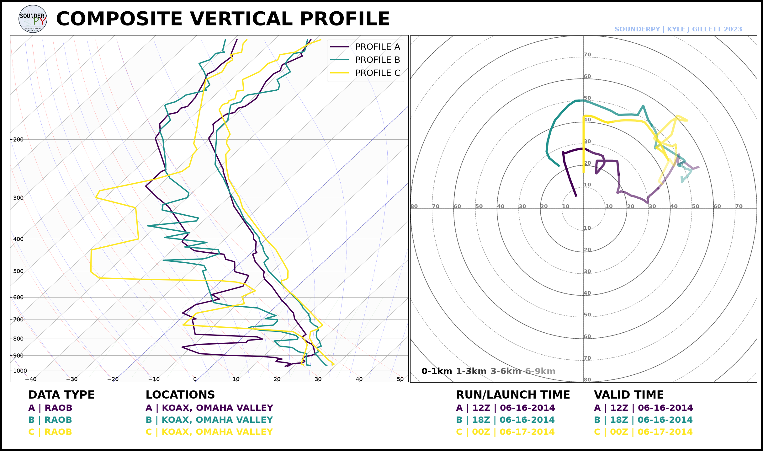
Create the comparison with:

spy.build_composite(
    profiles,
    shade_between=False,
)

Dark-Mode Composite

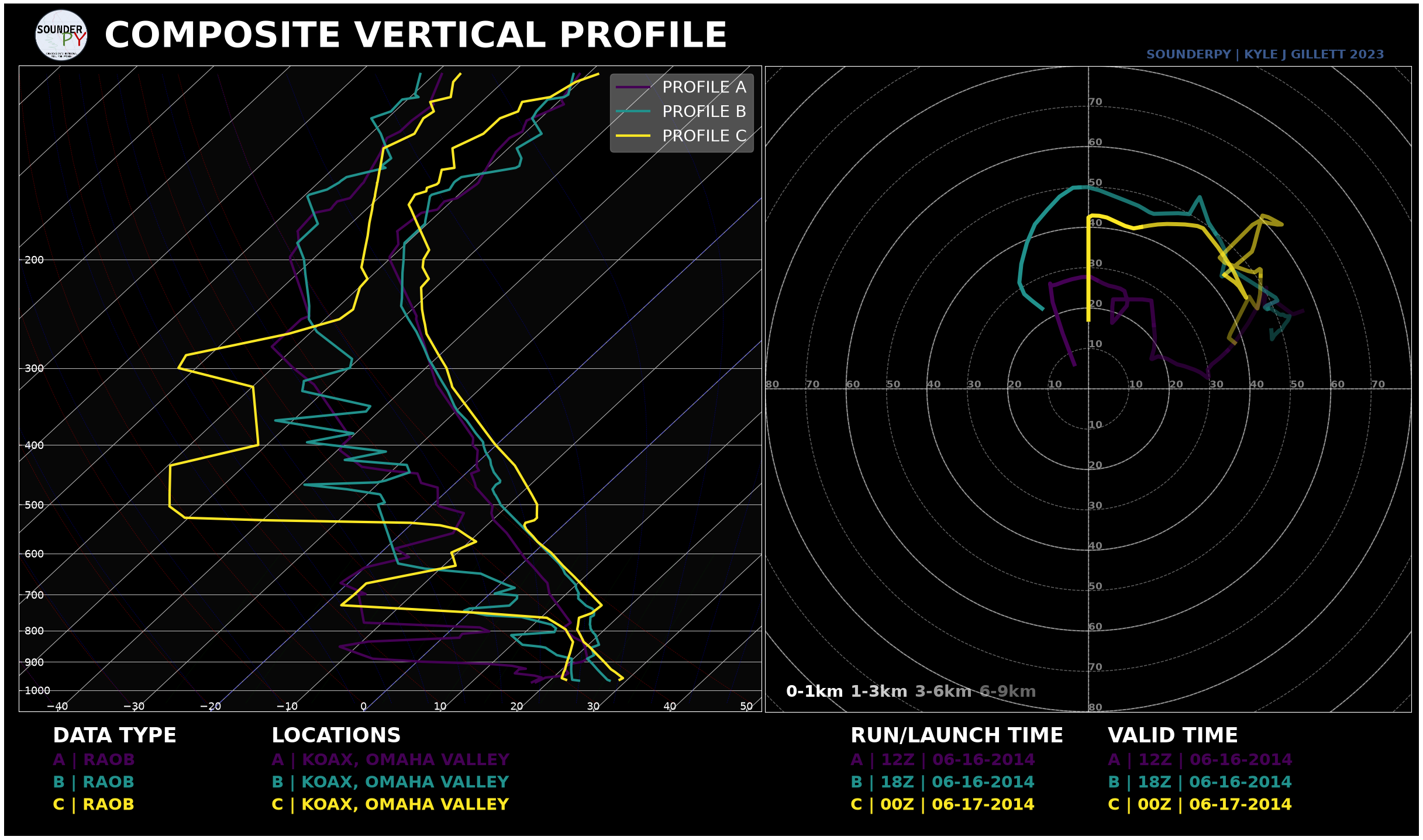
spy.build_composite(
    profiles,
    shade_between=False,
    dark_mode=True,
)

Shading between Temperature and Dewpoint

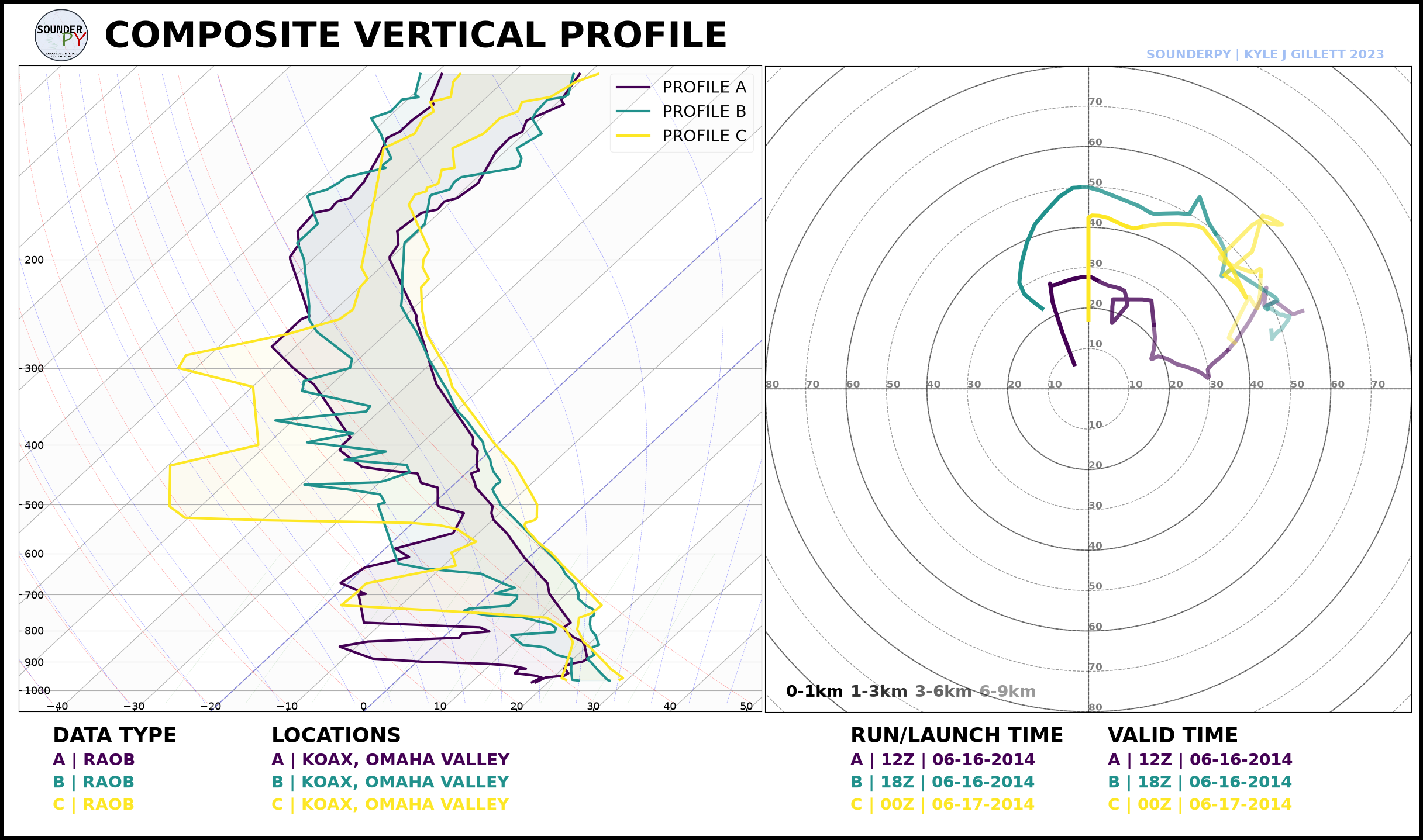
shade_between=True lightly shades the region between each profile’s temperature and dewpoint traces:

spy.build_composite(
    profiles,
    shade_between=True,
)

SounderPy composite sounding with shading

Choosing a Colormap

By default, SounderPy samples colors from viridis. Any compatible Matplotlib colormap can be supplied:

spy.build_composite(
    profiles,
    cmap="plasma",
)

or:

spy.build_composite(
    profiles,
    cmap="coolwarm",
)

Custom Colors

Provide one color for each profile with colors_to_use:

spy.build_composite(
    profiles,
    colors_to_use=[
        "tab:blue",
        "tab:orange",
        "tab:red",
    ],
)

If custom colors are supplied, the list length should match the number of profiles.

Line Styles

Line styles can also be assigned profile-by-profile:

spy.build_composite(
    profiles,
    ls_to_use=[
        "--",
        "-",
        ":",
    ],
)

Line Widths

spy.build_composite(
    profiles,
    lw_to_use=[
        2,
        4,
        2,
    ],
)

Opacity

spy.build_composite(
    profiles,
    alphas_to_use=[
        0.6,
        1.0,
        0.6,
    ],
)

Combine Styling Options

For example, emphasize the middle profile:

spy.build_composite(
    profiles,
    colors_to_use=[
        "tab:blue",
        "tab:red",
        "tab:purple",
    ],
    ls_to_use=[
        "--",
        "-",
        "--",
    ],
    lw_to_use=[
        2,
        4,
        2,
    ],
    alphas_to_use=[
        0.6,
        1.0,
        0.6,
    ],
    shade_between=False,
)

Compare Different Data Sources

Composite inputs do not have to come from the same source.

For example:

profiles = [
    observed_data,
    rap_data,
    bufkit_data,
]

spy.build_composite(
    profiles,
    colors_to_use=[
        "black",
        "tab:blue",
        "tab:orange",
    ],
)

Because each source has already been converted into clean_data, build_composite() can treat them consistently.

Save the Figure

spy.build_composite(
    profiles,
    shade_between=False,
    save=True,
    filename="oax_composite.png",
)

Next Steps

Continue to Exporting Data to save retrieved profiles for other software and workflows.