📊 Plot Gallery

SounderPy can create sounding, hodograph, composite, and VAD-based visualizations from observed, forecast, reanalysis, model-output, and custom vertical profile data.

Most comparison examples use the same observed OAX sounding from 16 June 2014 at 18 UTC so that visual differences reflect plotting options rather than differences in the atmospheric profile.

Light and Dark Themes

The same SounderPy profile can be rendered using either the default light appearance or the dark-background plotting style.

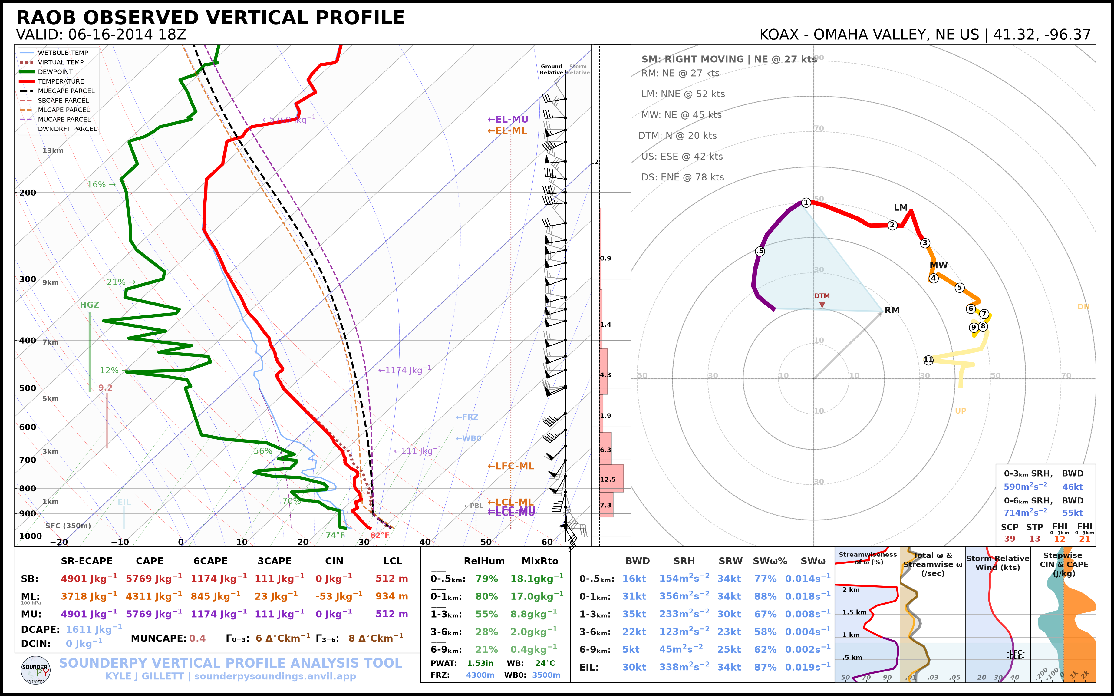
Light-Mode Sounding

Default SounderPy appearance.

spy.build_sounding(
    data,
    dark_mode=False,
)

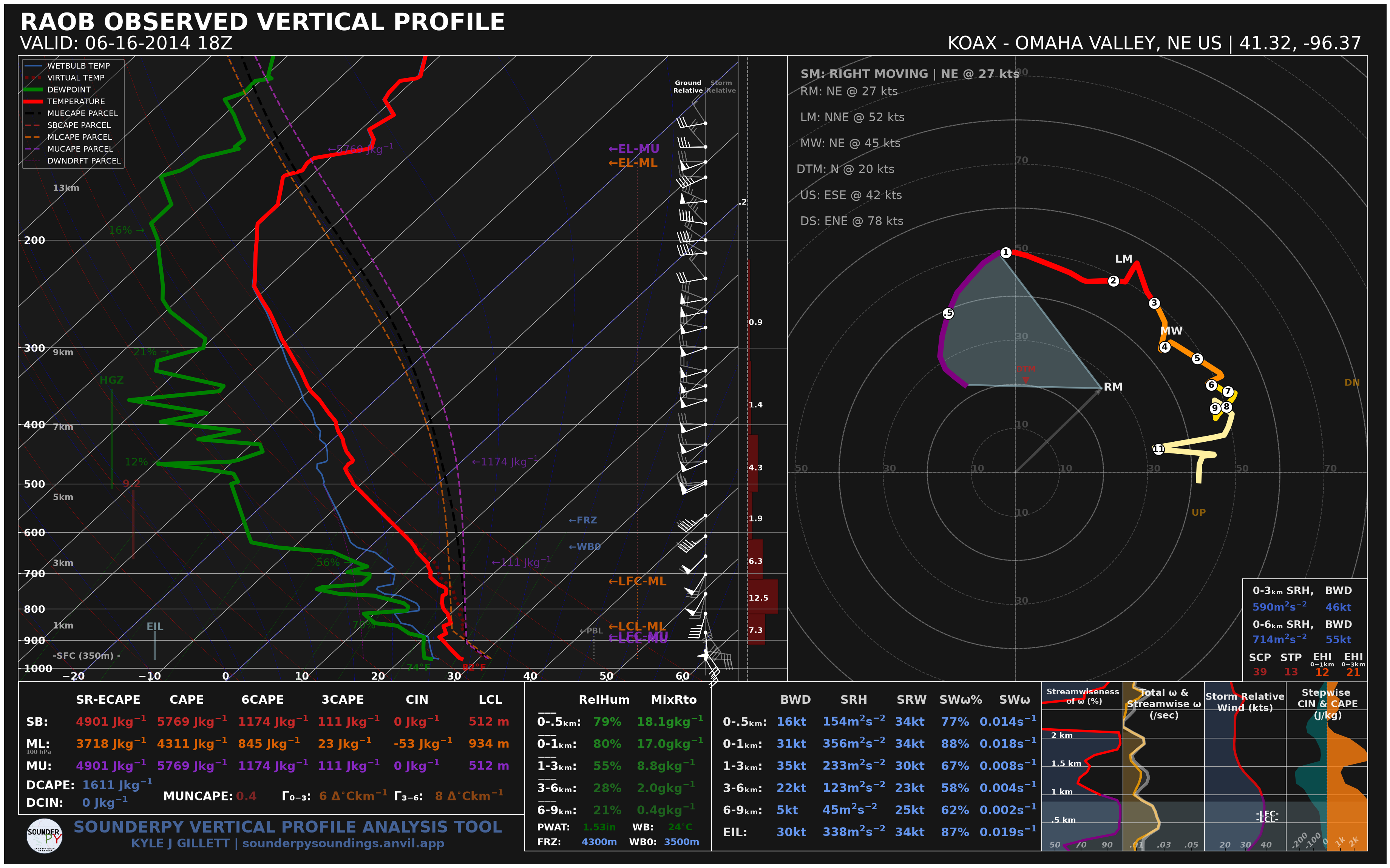
Dark-Mode Sounding

Enable the dark-mode with: dark_mode=True.

spy.build_sounding(
    data,
    dark_mode=True,
)

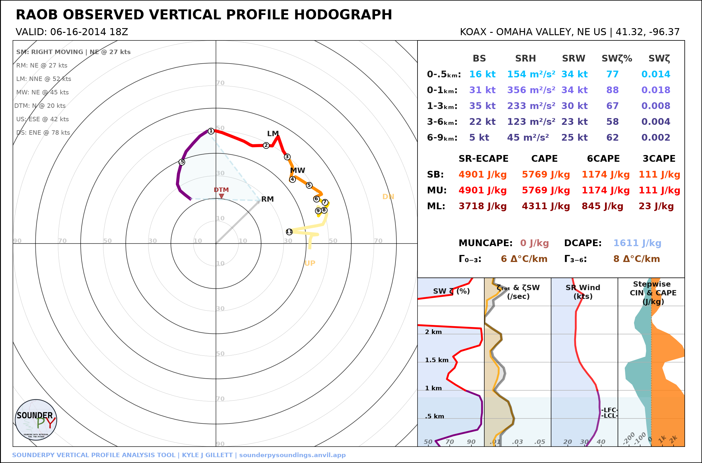
Light-Mode Hodograph

spy.build_hodograph(
    data,
    dark_mode=False,
)

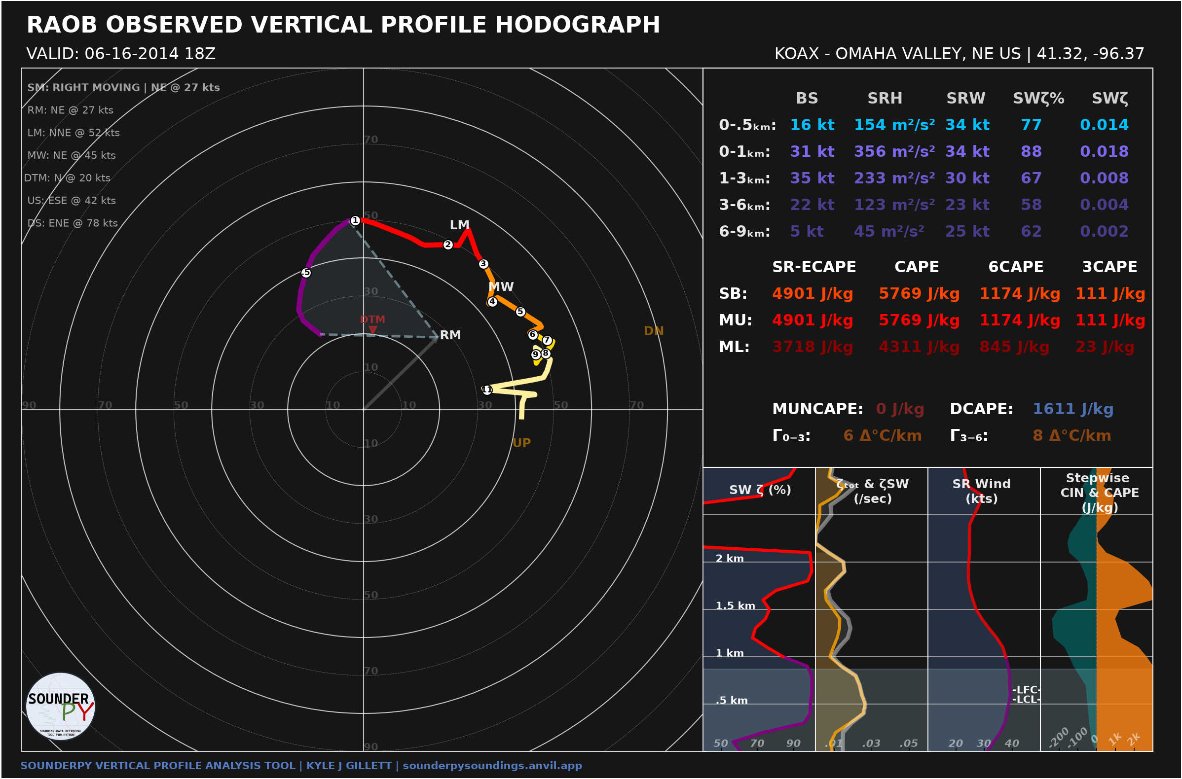
Dark-Mode Hodograph

spy.build_hodograph(
    data,
    dark_mode=True,
)

Color-Deficiency-Friendly Settings

SounderPy includes a color-deficiency-friendly option for sounding plots. This simply changes the dewpoint trace from green to blue.

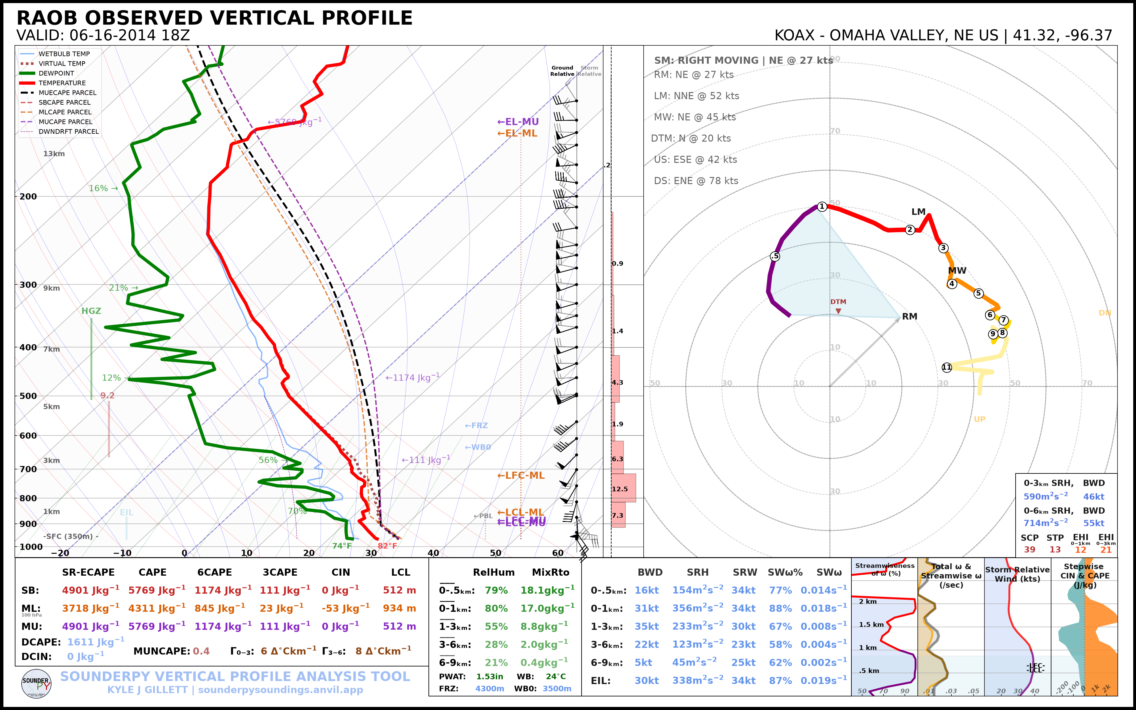
Standard Colors

spy.build_sounding(
    data,
    color_blind=False,
)

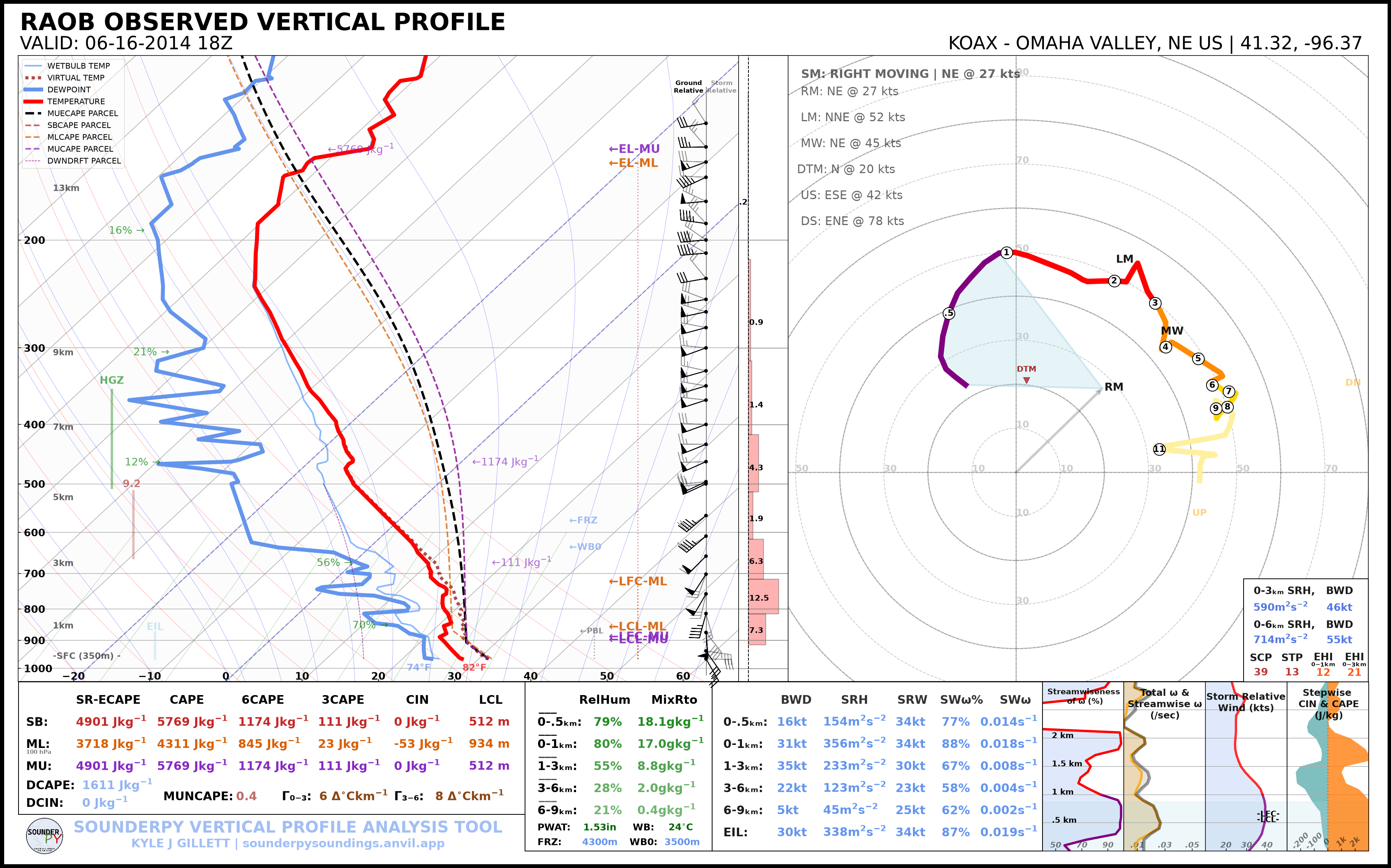
Color-Deficiency-Friendly

spy.build_sounding(
    data,
    color_blind=True,
)

Map and Radar Settings

The SounderPy map inset can be disabled, displayed without radar, or combined with supported radar data.

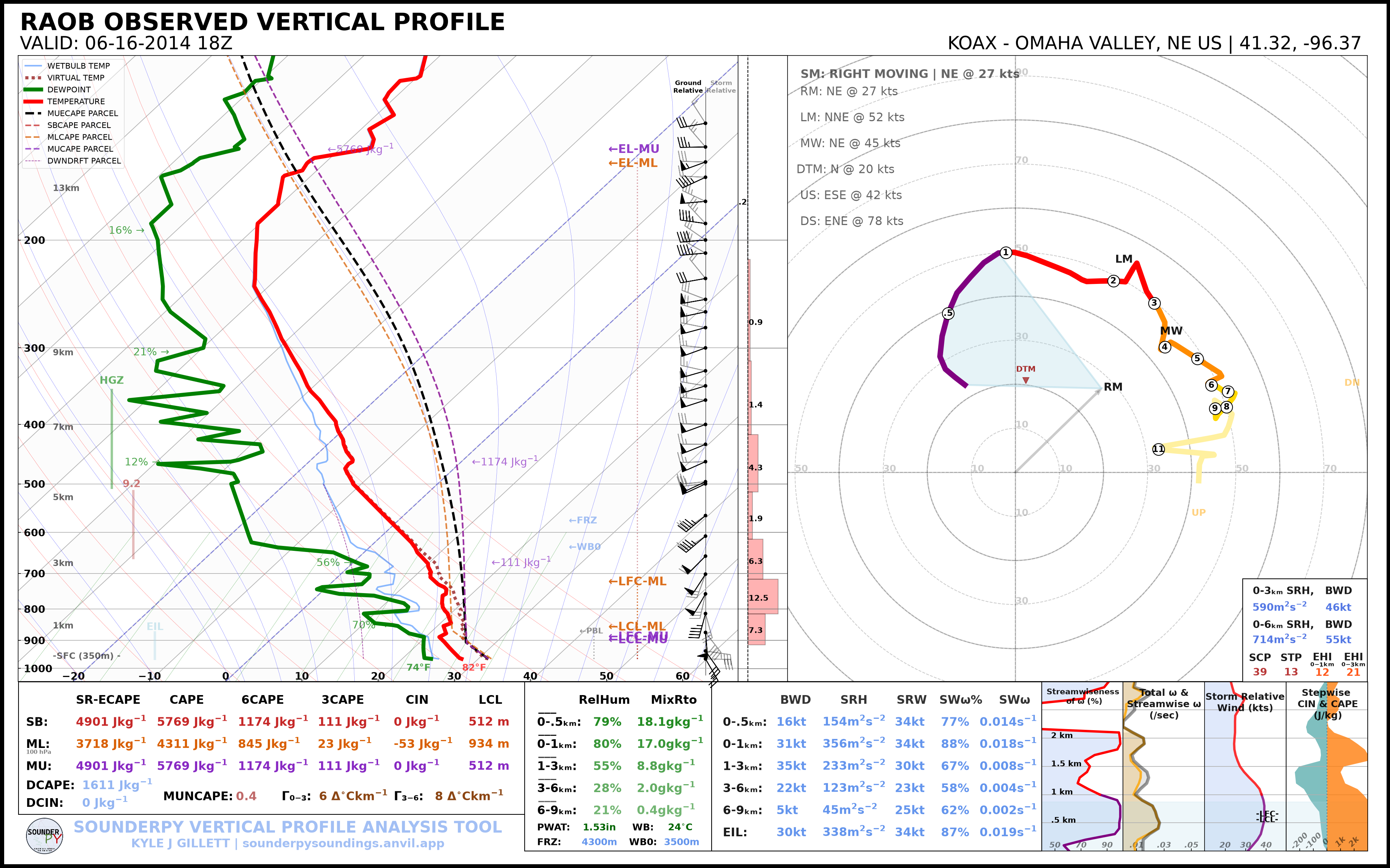
Map Disabled

Set map_zoom=0 to remove the map inset.

spy.build_sounding(
    data,
    radar=None,
    map_zoom=0,
)

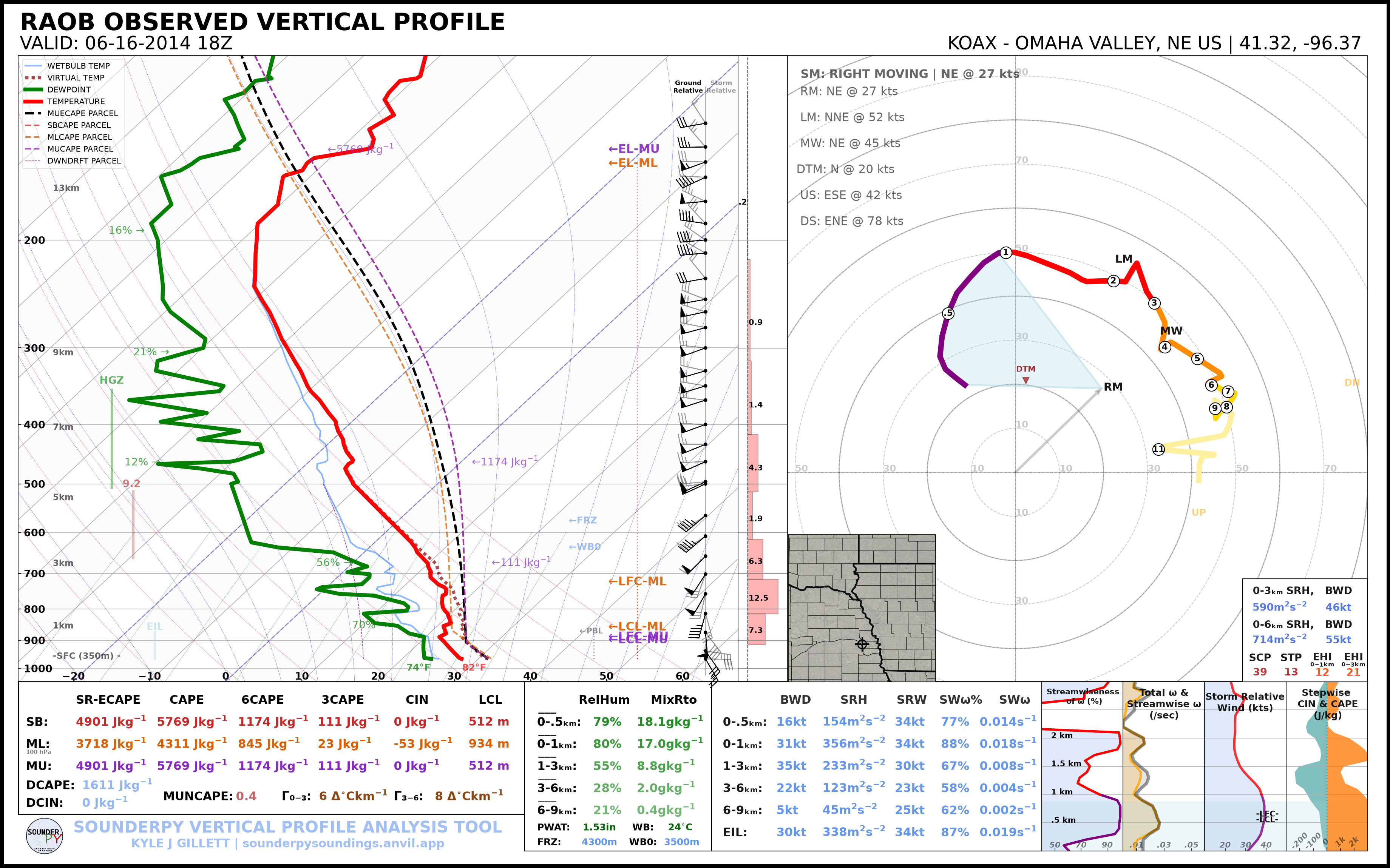
SounderPy sounding with map enabled and radar disabled

Map Only

Display the map while disabling radar.

spy.build_sounding(
    data,
    radar=None,
    map_zoom=2,
)

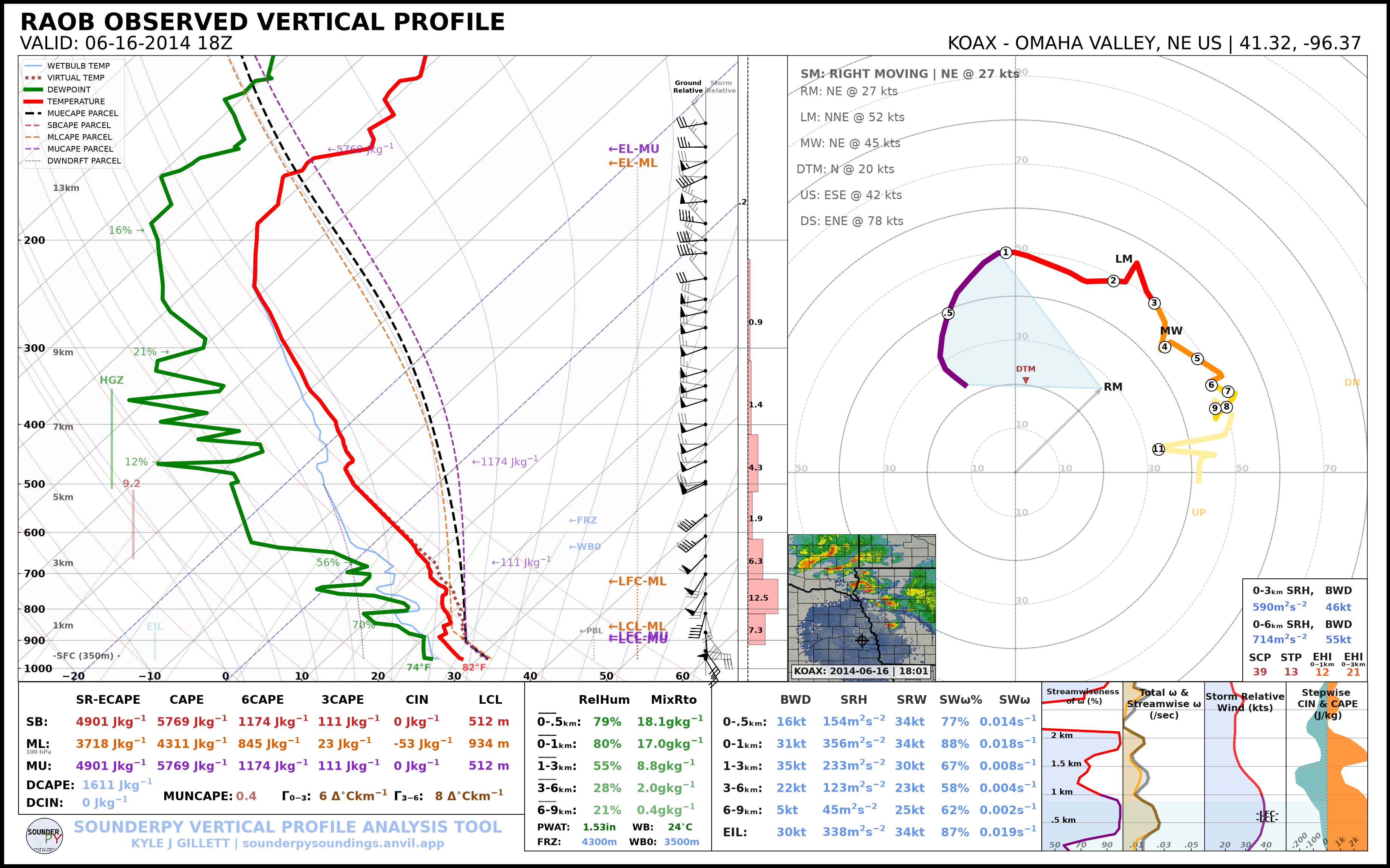
Single-Site Radar

Use WSR-88D data from the nearest radar site.

spy.build_sounding(
    data,
    radar="single",
    radar_time="sounding",
    map_zoom=2,
)

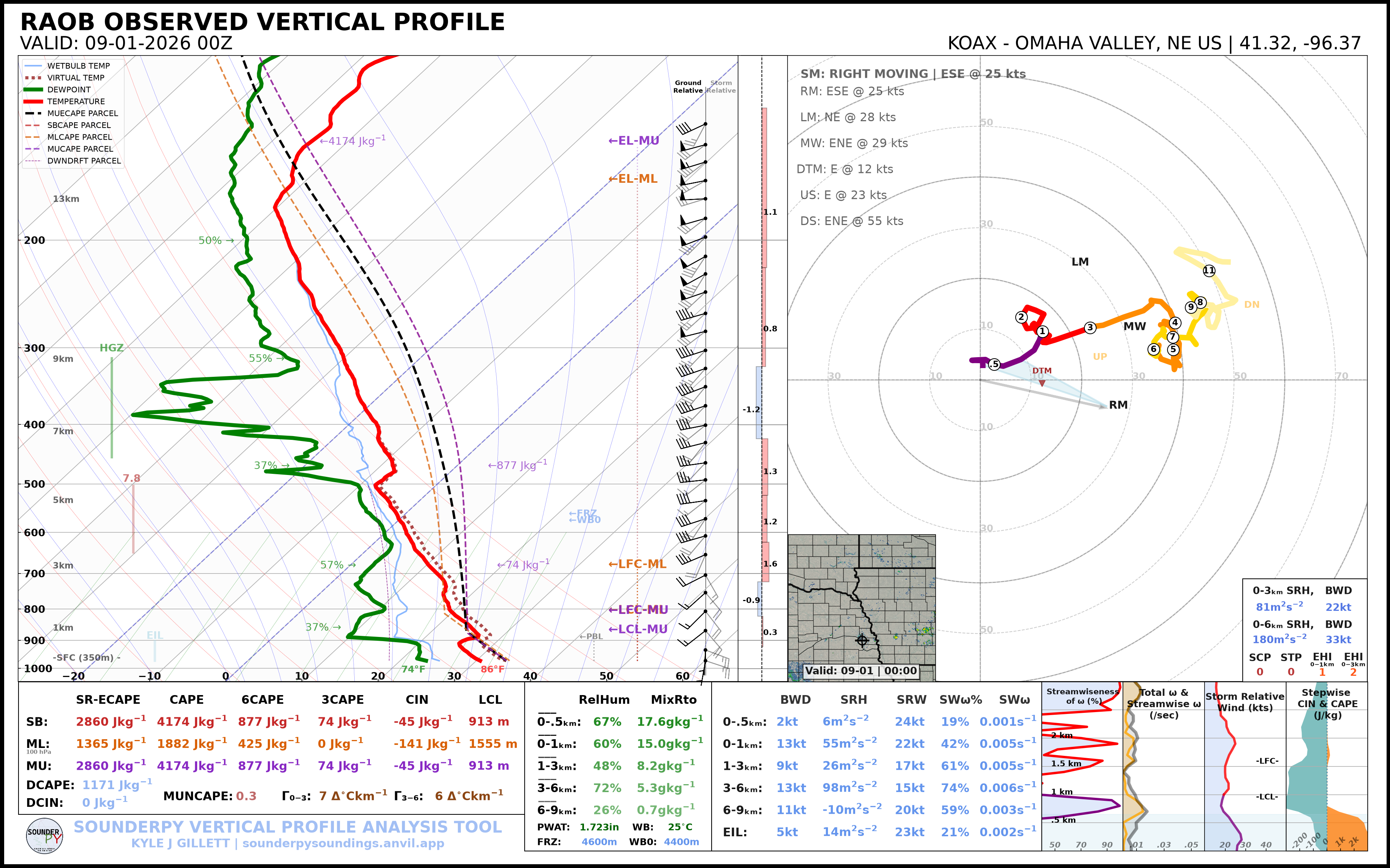
Radar Mosaic

Use recent CONUS mosaic reflectivity data.

spy.build_sounding(
    data,
    radar="mosaic",
    radar_time="sounding",
    map_zoom=2,
)

Map Zoom

The map extent can also be changed with map_zoom. A larger integer will zoom out (including more of the map).

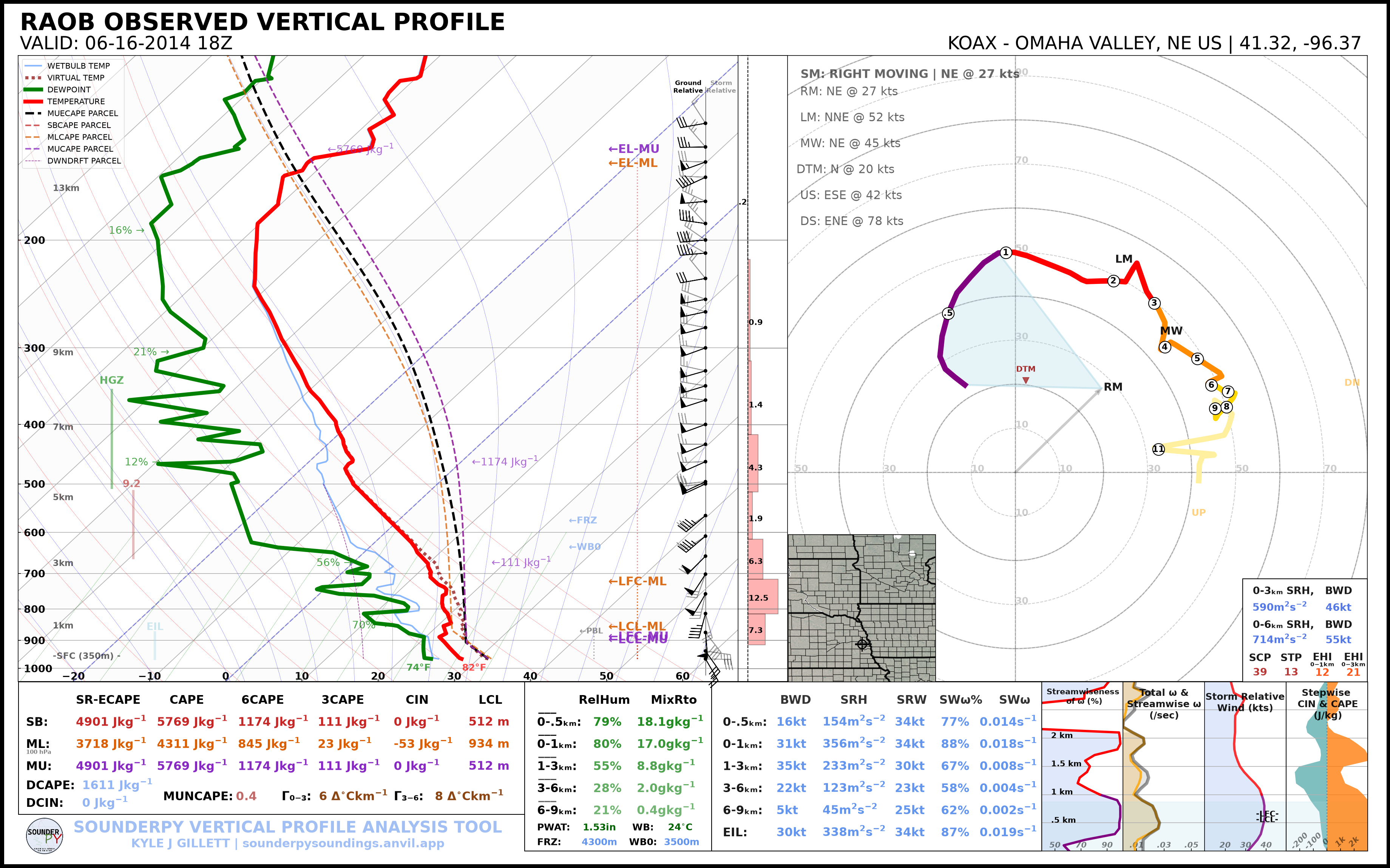
SounderPy sounding with a larger map extent

spy.build_sounding(
    data,
    radar=None,
    map_zoom=4,
)

Parcel Settings

SounderPy supports default parcel behavior, a simplified parcel configuration, and custom parcel highlighting/background combinations.

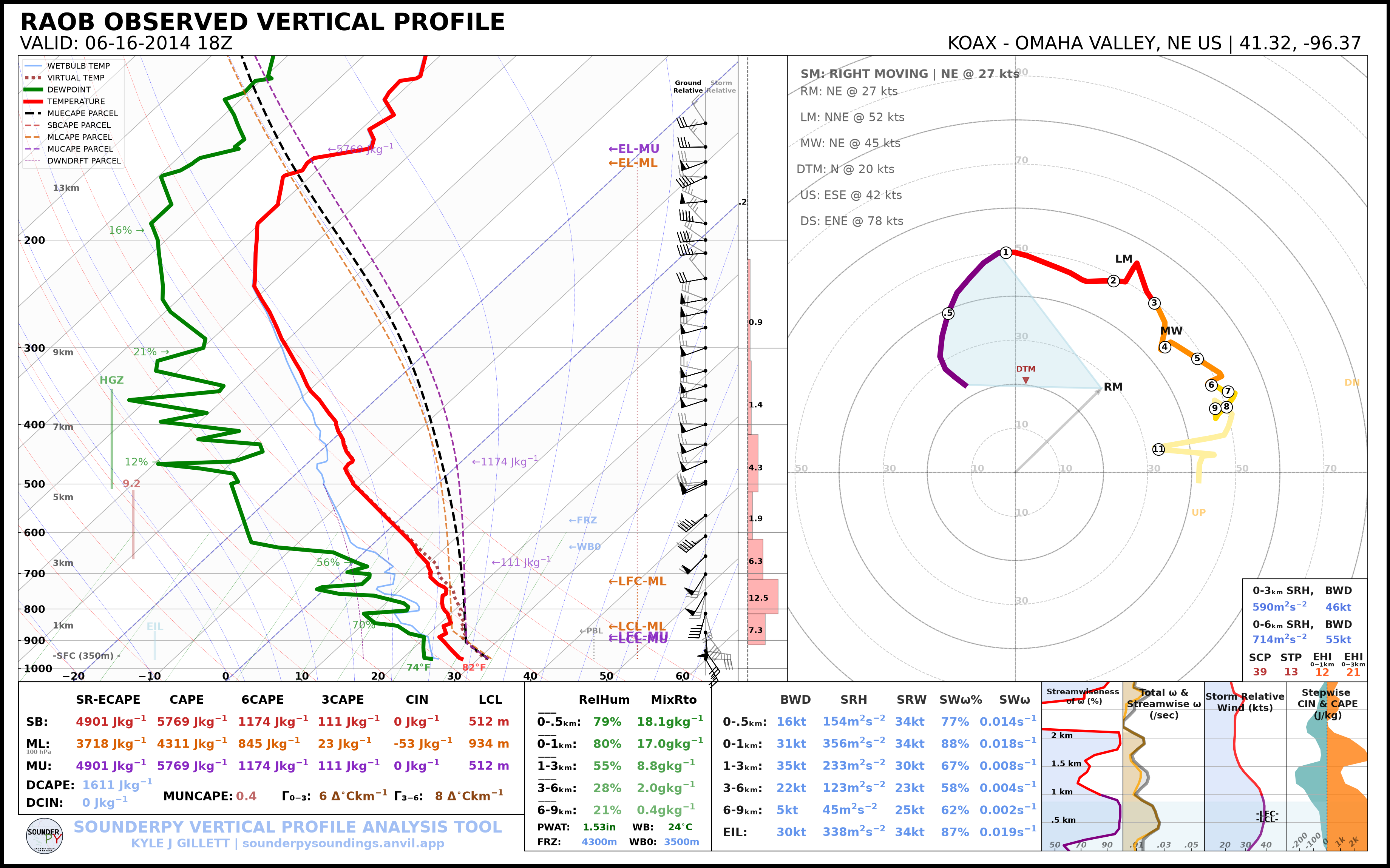
Default Parcels

Use SounderPy’s standard parcel configuration.

spy.build_sounding(
    data,
    special_parcels=None,
)

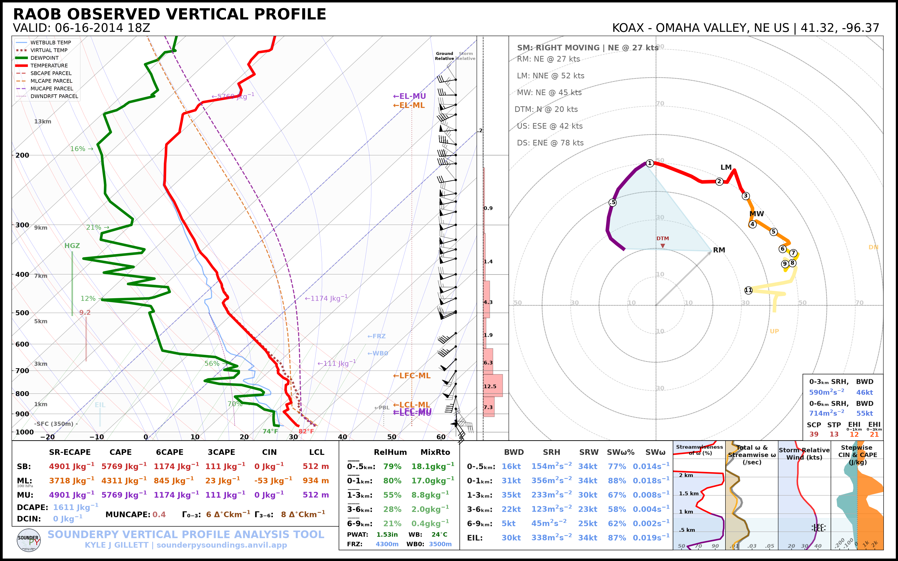
Simple Parcels

Use the simplified parcel configuration.

spy.build_sounding(
    data,
    special_parcels="simple",
)

Custom Parcel Configuration

Custom parcel settings allow selected parcel types to be highlighted while others are displayed in the background.

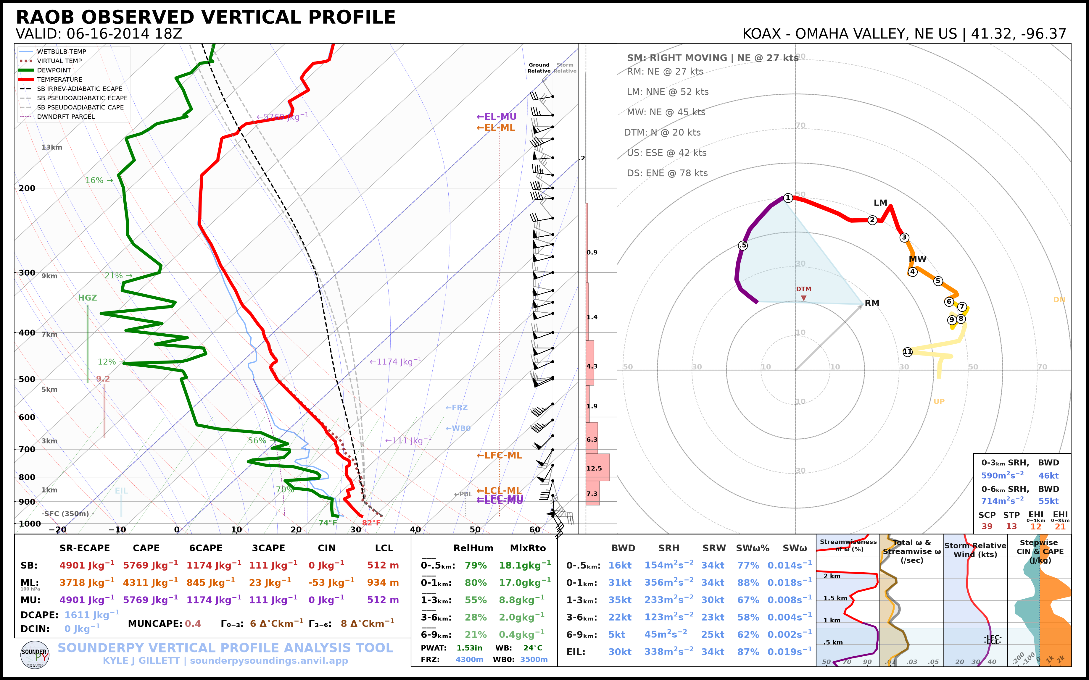
SounderPy sounding using custom parcel settings

For example:

custom_parcels = [
    ["sb_ia_ecape"],
    ["sb_ps_ecape", "sb_ps_cape"],
]

spy.build_sounding(
    data,
    special_parcels=custom_parcels,
)

Additional Plot Options

Theta and Theta-e

If you’d like to maintain the classic low-level theta and theta-e profiles, you may do so by using show_theta=True:

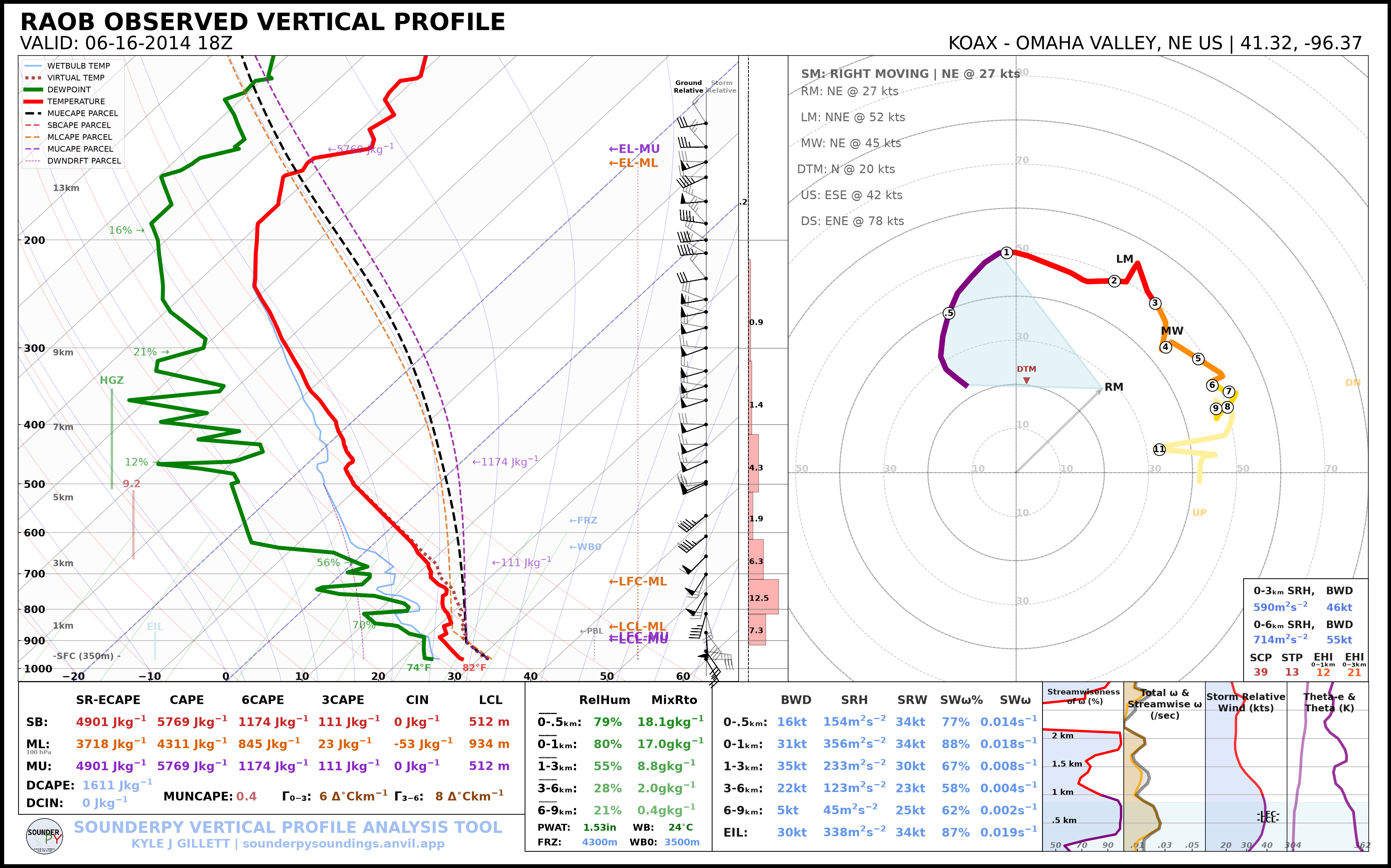
spy.build_sounding(data, show_theta=True)

Ground-Relative vs Storm-Relative Hodographs

You may translate hodograph data to a storm-relative reference frame with sr_hodo=True. This may be done for hodograph and sounding plots.

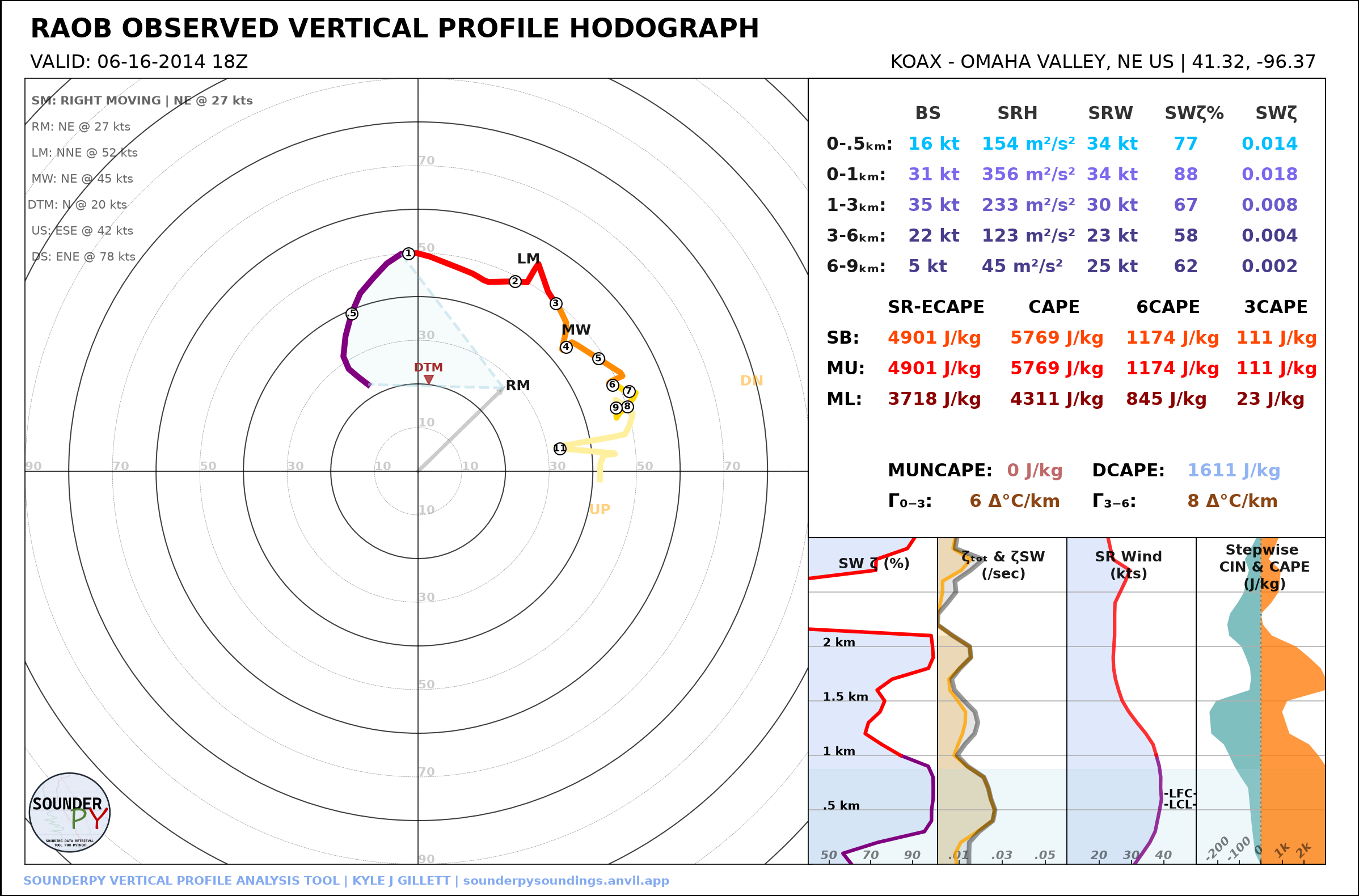
Ground Relative

spy.build_hodograph(
    data,
    sr_hodo=False,
)

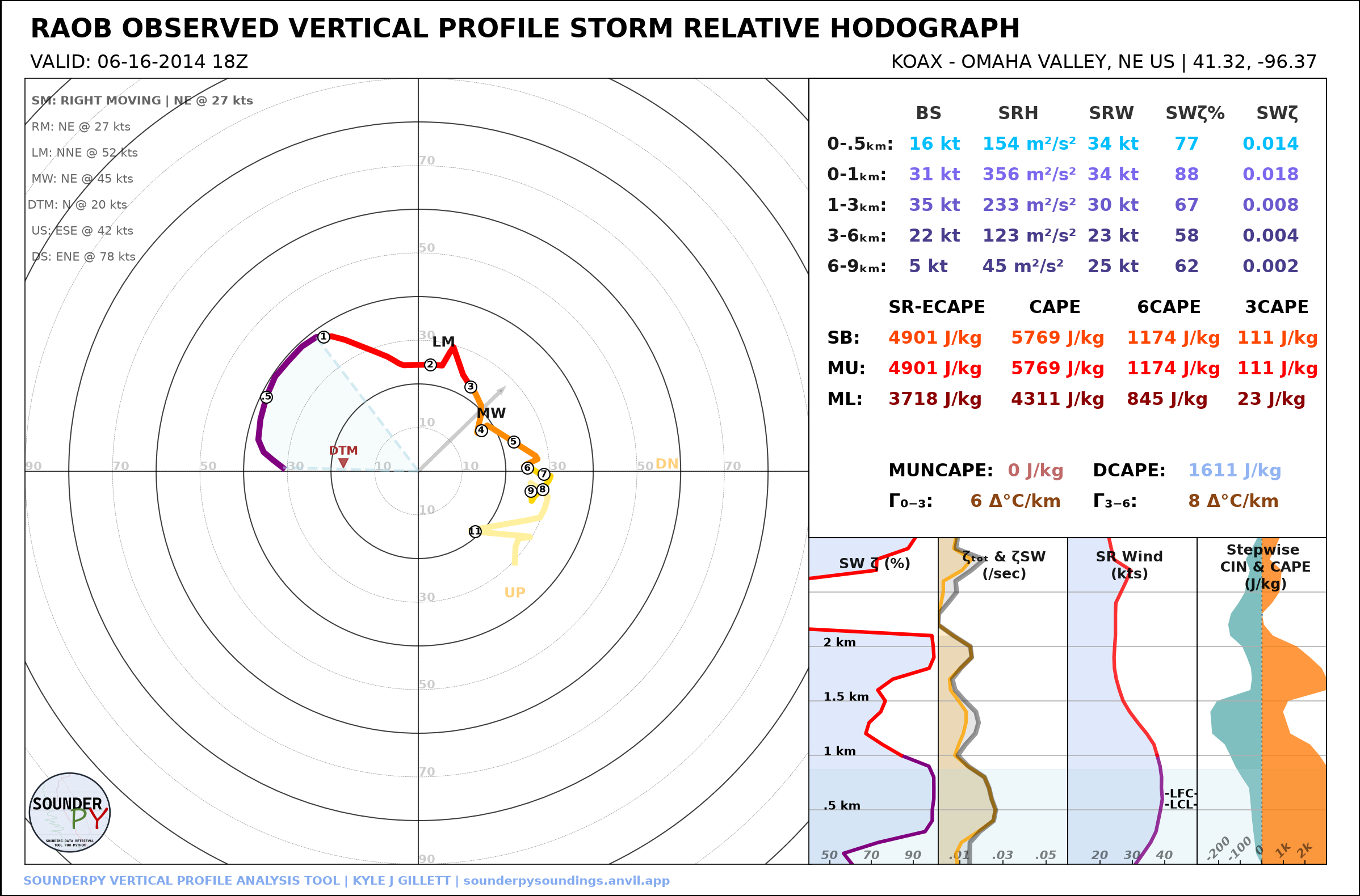
Storm Relative

spy.build_hodograph(
    data,
    sr_hodo=True,
)

Custom Storm Motion

You can set a custom storm motion using storm_motion = [direction, speed]. This may be done for hodograph and sounding plots.

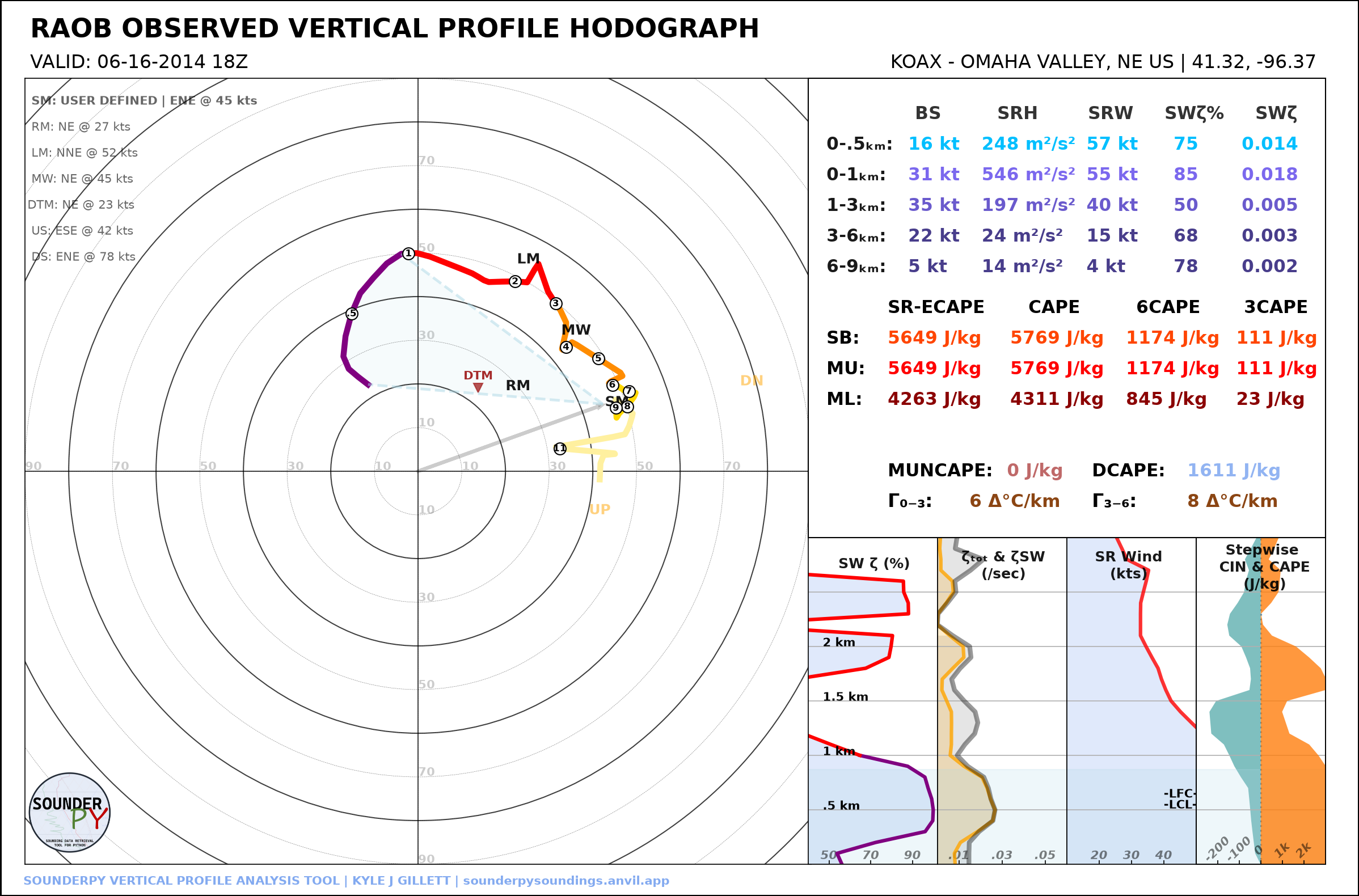
spy.build_hodograph(data, storm_motion=[250.0, 45.0])

Hodograph Boundary

Here you can add a line to the hodograph plot to visualize the orientation of the flow relative to a nearby boundary (such as a cold front, outflow boundary, etc). This may be done for hodograph and sounding plots.

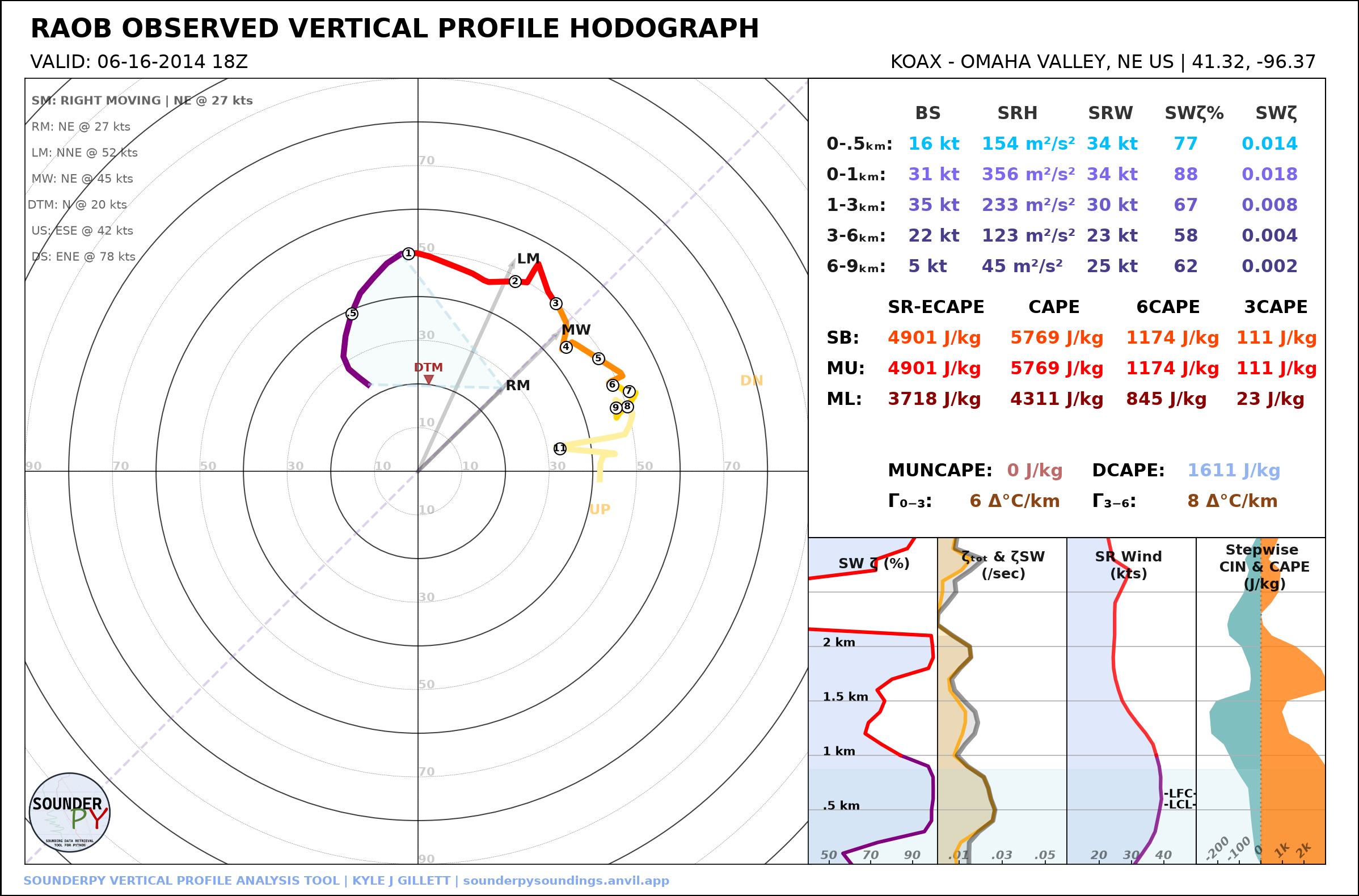
SounderPy hodograph with a custom boundary line

spy.build_hodograph(data, hodo_boundary={"angle": [45], "color": ["tab:purple"]})

Different Data Sources

One of SounderPy’s core design features is that vertical profiles from many different sources are converted into the same clean_data structure. Once a profile has been retrieved or converted, the same plotting functions can be used regardless of its source.

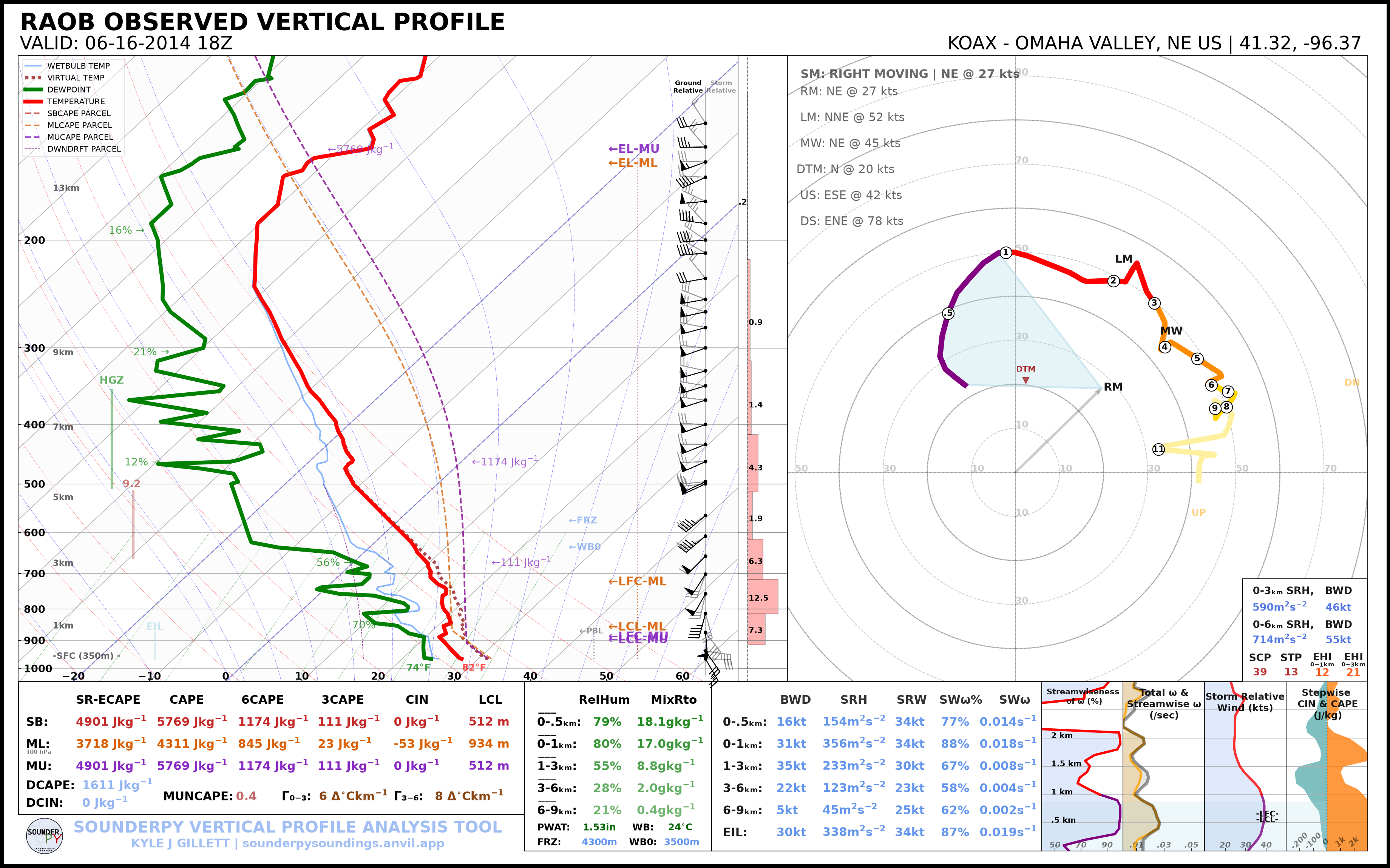
Observed RAOB

data = spy.get_obs_data(
    "OAX",
    "2014", "06", "16", "18",
)

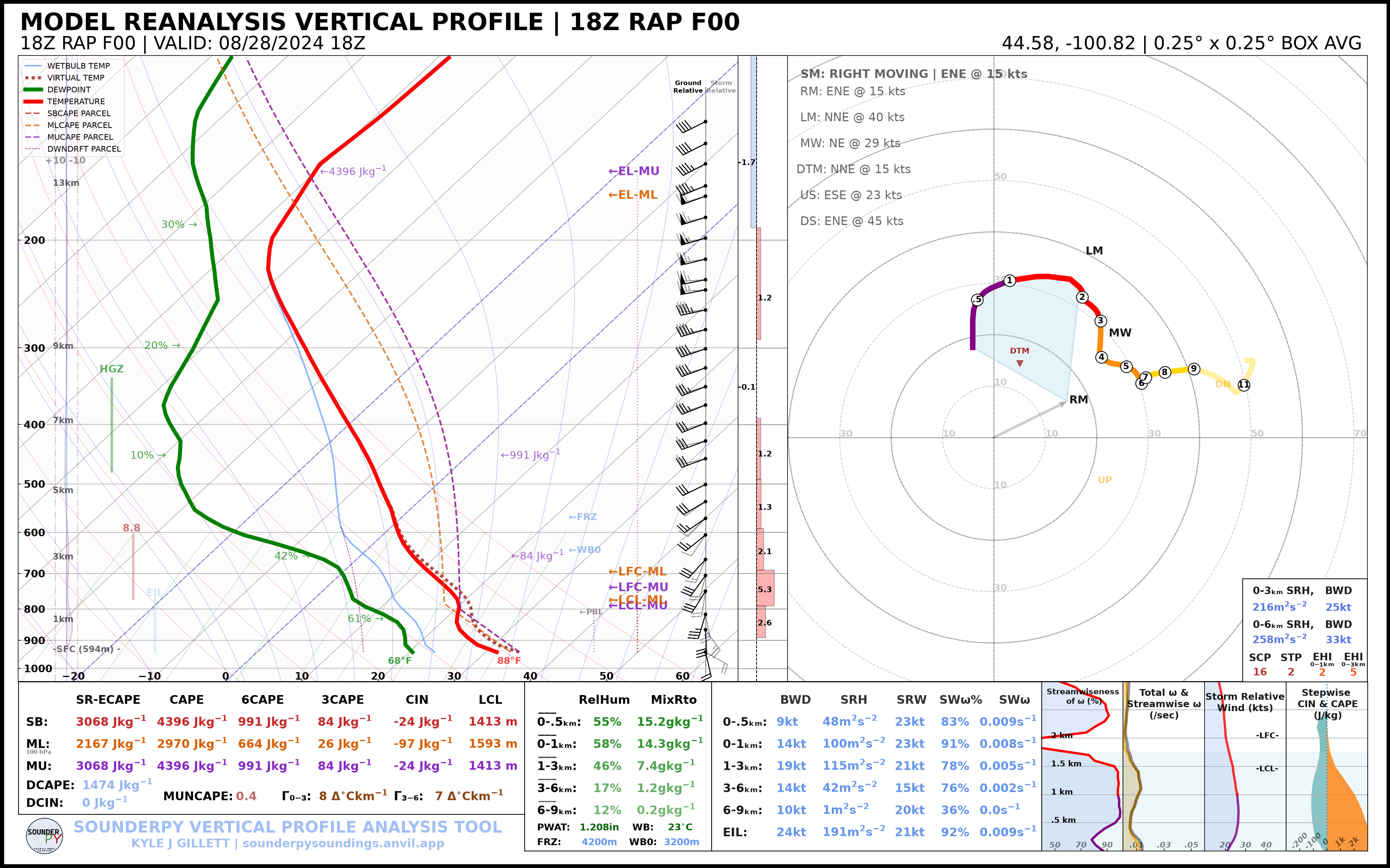
RAP/RUC Reanalysis

data = spy.get_model_data("rap-ruc",
    [44.58, -100.82],
    "2024", "08", "28", "18",
    box_avg_size=0.25)

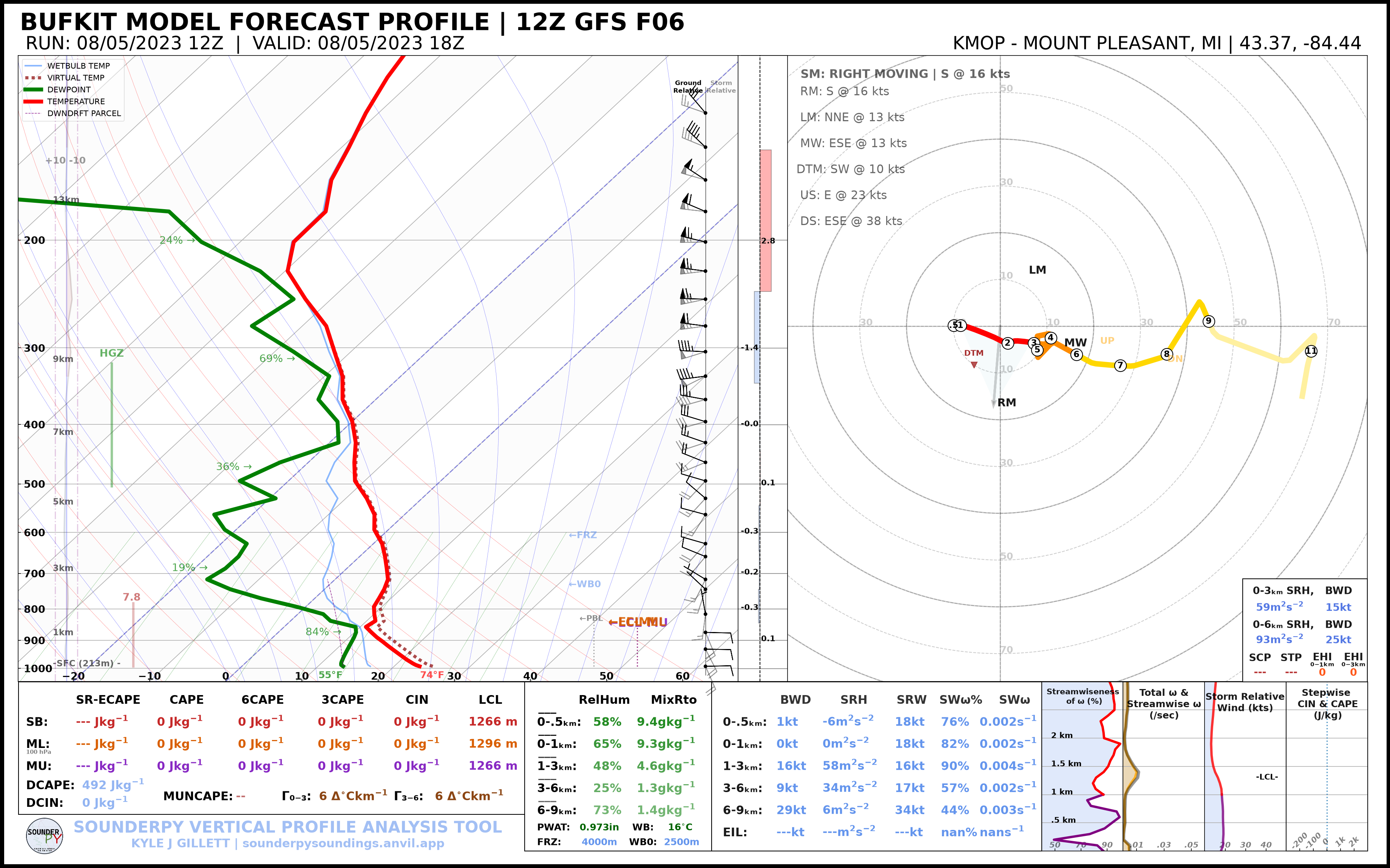
BUFKIT Forecast

data = spy.get_bufkit_data(
    "gfs",
    "KMOP",
    6,
    "2023", "08", "05", "12",
)

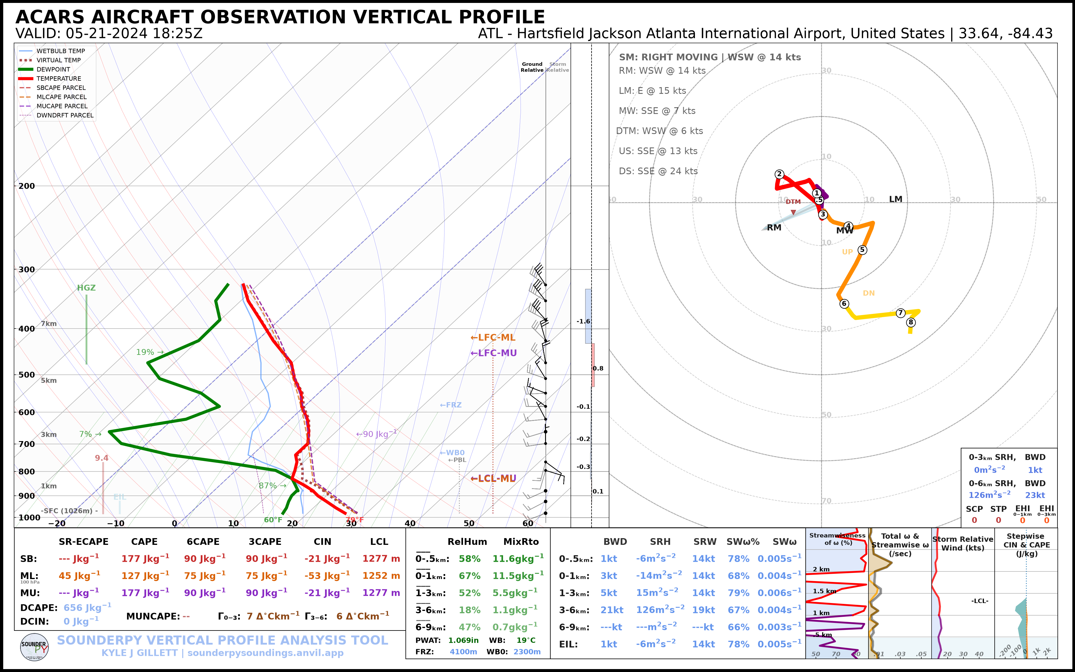
SounderPy sounding using ACARS aircraft data

ACARS Aircraft Profile

conn = spy.acars_data(
    "2024", "05", "21", "18",
)

profiles = conn.list_profiles()
data = conn.get_profile(profiles[0])

The same approach also applies to ERA5, NCEP, WRF, CM1, and user-created custom profiles.

See Getting Data and Custom Data Sources for additional information.

Composite Soundings

Composite plots are useful for comparing temporal evolution, model forecasts, observations versus reanalysis, or other groups of profiles.

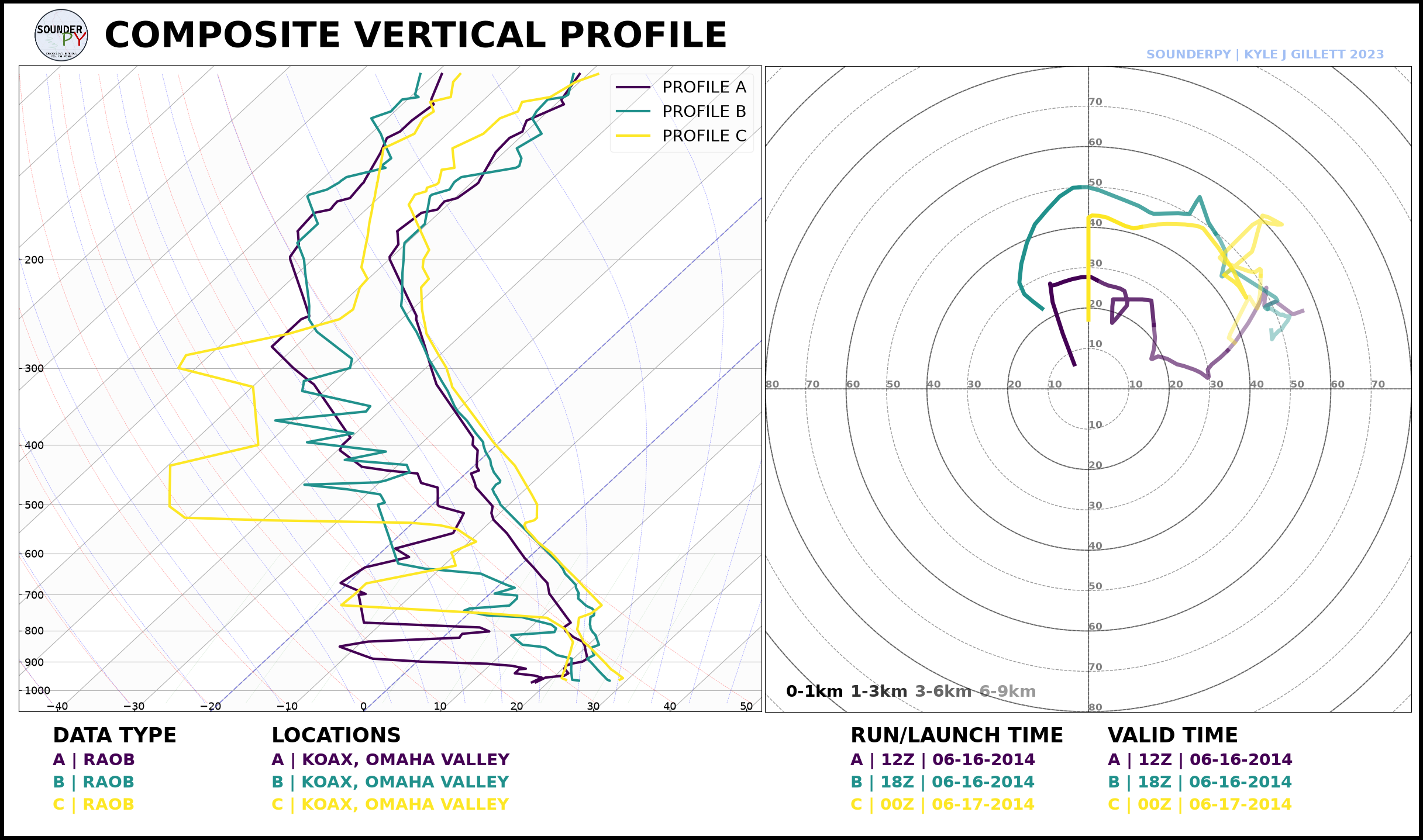
Light Composite

A standard multi-profile comparison.

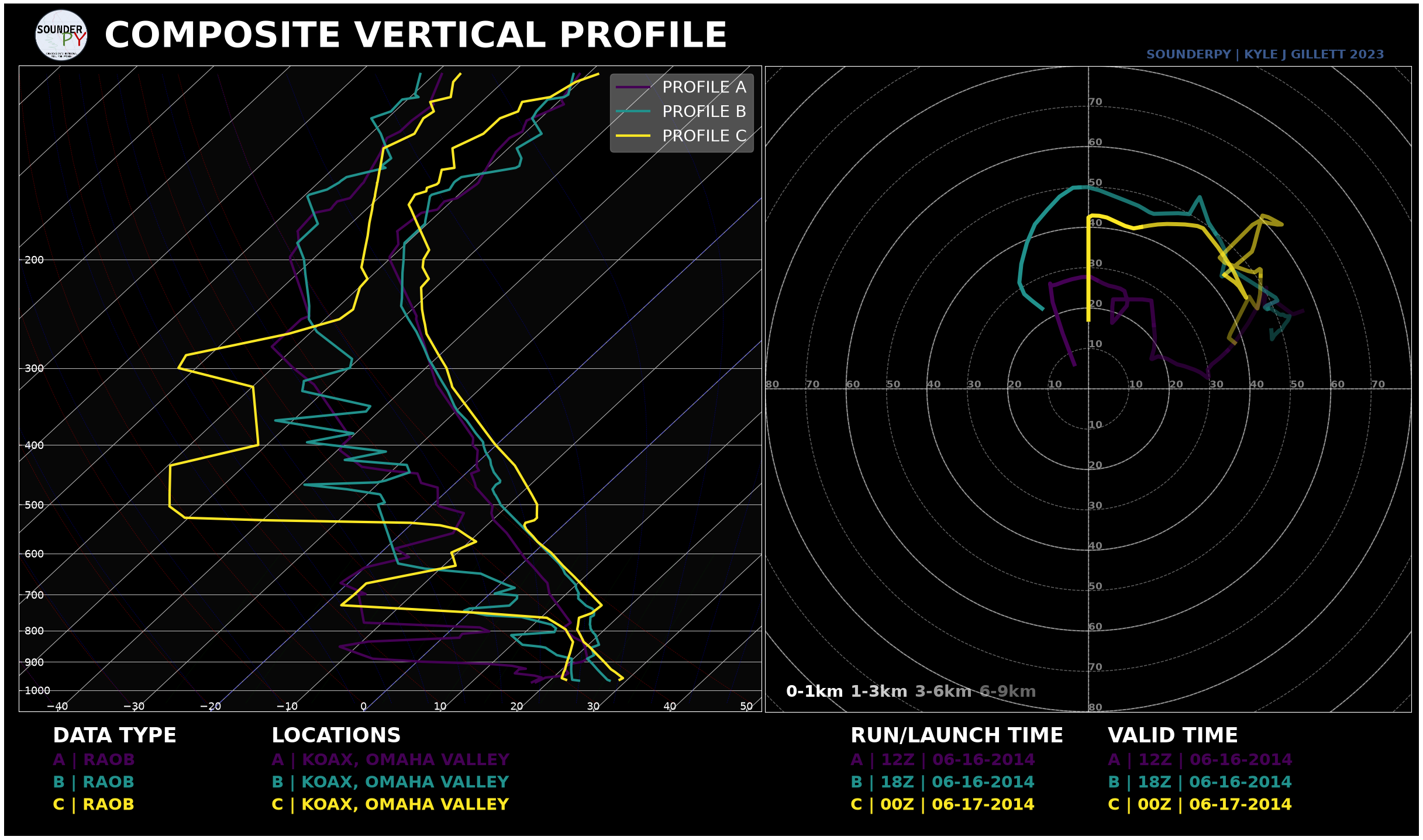
Dark Composite

With dark_mode=True.

SounderPy composite sounding with shading

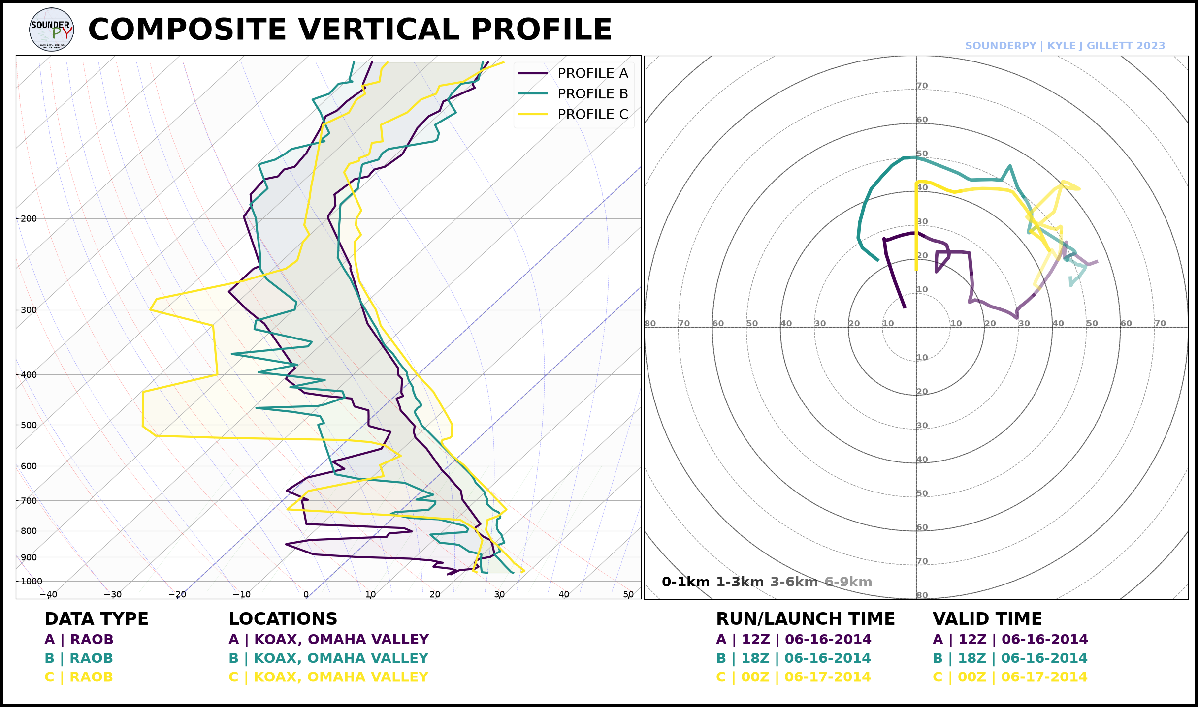
Shaded Composite

With shade_between=True.

Continue Learning

For detailed explanations and additional examples, see: