📈 Tools for Plotting Data
Initially, SounderPy was a tool meant for getting and parsing data with not as much focus on plotting said data. However, recent releases have put more emphasis on plotting capabilites. Version 3.0.0+ features a number of significant & exciting upgrades to SounderPy’s plotting abilities.
SounderPy can create general sounding and hodograph plots as well as composite sounding plots!
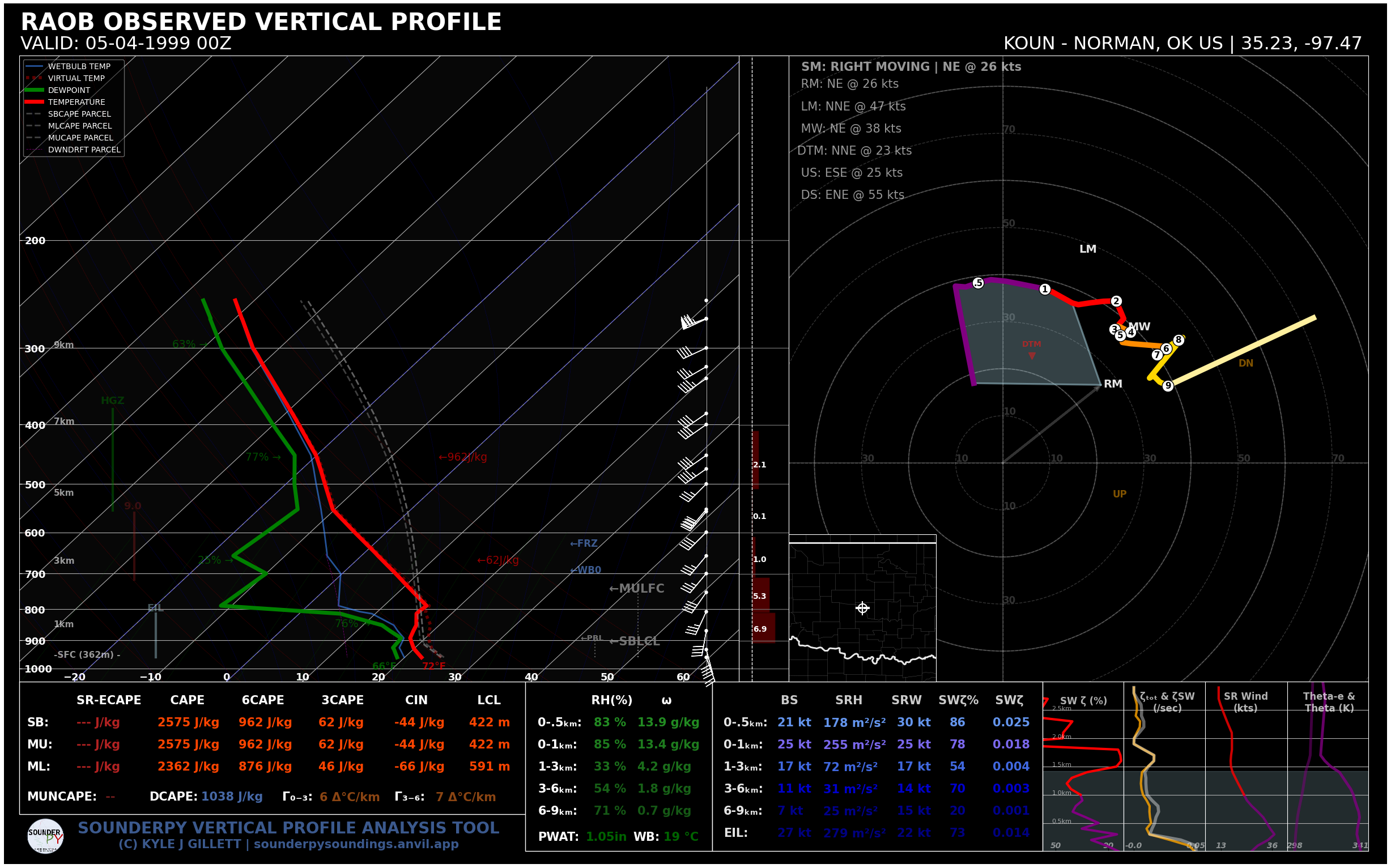
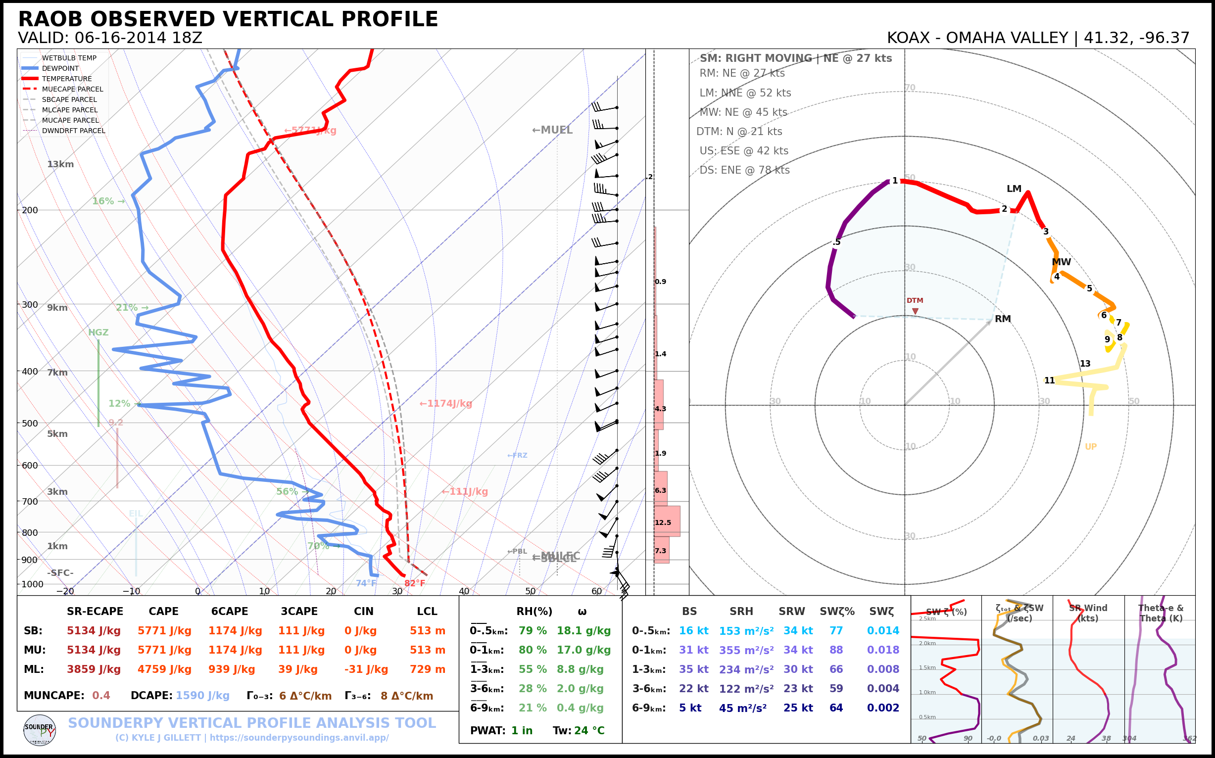
The full sounding plot that SounderPy creates is a complex figure with unique design geared towards severe convective storm enviroment analysis.
These sounding plots are ‘my baby’ and I hope you find them useful! :)
Check out SounderPy’s 📊 Plot Gallery & 📝 Usage Examples
Tip
Do your plots have funky scaling? This is a common issue for smaller screen sizes. To fix this, use the save=True kwarg in your plot function.
Building Soundings
While this function may appear complicated at first glance, there is actually only one required argument for this function. The other arguments are simply optional settings for the plot!
- spy.build_sounding(clean_data, color_blind=False, dark_mode=False, storm_motion='right_moving', special_parcels=None, radar='mosaic', radar_time='sounding', map_zoom=2, modify_sfc=None, show_theta=False, hodo_boundary=None, save=False, filename='sounderpy_sounding')
Return a full sounding plot of SounderPy data,
plt- Parameters:
clean_data (dict, required) – the dictionary of data to be plotted (see 🌐 Tools for Getting Data)
color_blind (bool, optional, Default is
False) – whether or not to change the dewpoint trace line from green to blue for improved readability for color deficient users/readers.dark_mode (bool, optional, Default is
False.) –Truewill invert the color scheme for a ‘dark-mode’ sounding.storm_motion (str or list of floats, optional, Default is 'right_moving'.) – the storm motion used for plotting and calculations. Custom storm motions are accepted as a list of floats representing direction and speed. Ex:
[270.0, 25.0]where ‘270.0’ is the direction in degrees and ‘25.0’ is the speed in kts. See the Storm Motion Logic section for more details.special_parcels (nested list of two lists, optional, Default is None) – a nested list of special parcels from the
ecape_parcelslibrary. The nested list should be a list of two lists ([[a, b], [c, d]]) where the first list should include ‘highlight parcels’ and second list should include ‘background parcels’. For more details, see the Parcel Logic section. Another option is ‘simple’, which removes all advanced parcels making the plot quicker.radar (str,
"mosaic","single-site", orNone. Optional. Default ismosaic.) – whether to display mosaic reflectivity, single-site reflectivity, or no radar in the map inset.radar_time (str or datetime obj, optional, Default is
"sounding".) – radar mosaic data valid time. May be"sounding"(uses the valid time of the sounding data),``”now”`` (current time/date), or a datetime obj Note: radar mosaic data only goes back 1 month from current datemap_zoom (int, optional, Default is
2.) – a ‘zoom’ level for the map inset as an int. Note: Setting ``map_zoom=0`` will hide the mapmodify_sfc (None or dict, optional, default is None) – a dict in the format
{'T': 25, 'Td': 21, 'ws': 20, 'wd': 270}to modify the surface values of theclean_datadict. See the Surface Modification Logic section for more details.show_theta (bool, optional) – whether to replace the piecewise CAPE plot with theta & theta-e. Default is
Falsehodo_boundary (dict of lists – structured as
{'angle':[], 'color':[]}, optional) – plot a “boundary” (straight line) on the hodograph axis. Do so by providing an angle and a color. The angle represents the angle between zero-degrees (north) and the upper-half of the boundary line, to the right. Multiple boundaries can be plotted. Default isNonesave (bool, optional, Default is
False.) – whether to show the plot inline or save to a file.filename (str, optional, Default is sounderpy_sounding.) – the filename by which a file should be saved to if
save = True.
- Returns:
plt, a SounderPy sounding figure.
- Return type:
plt
Example
import sounderpy as spy

# get data | Note: any sounderpy data will work!
clean_data = spy.get_obs_data('OAX', '2014', '06', '16', '18')

# build the sounding!
spy.build_sounding(clean_data)
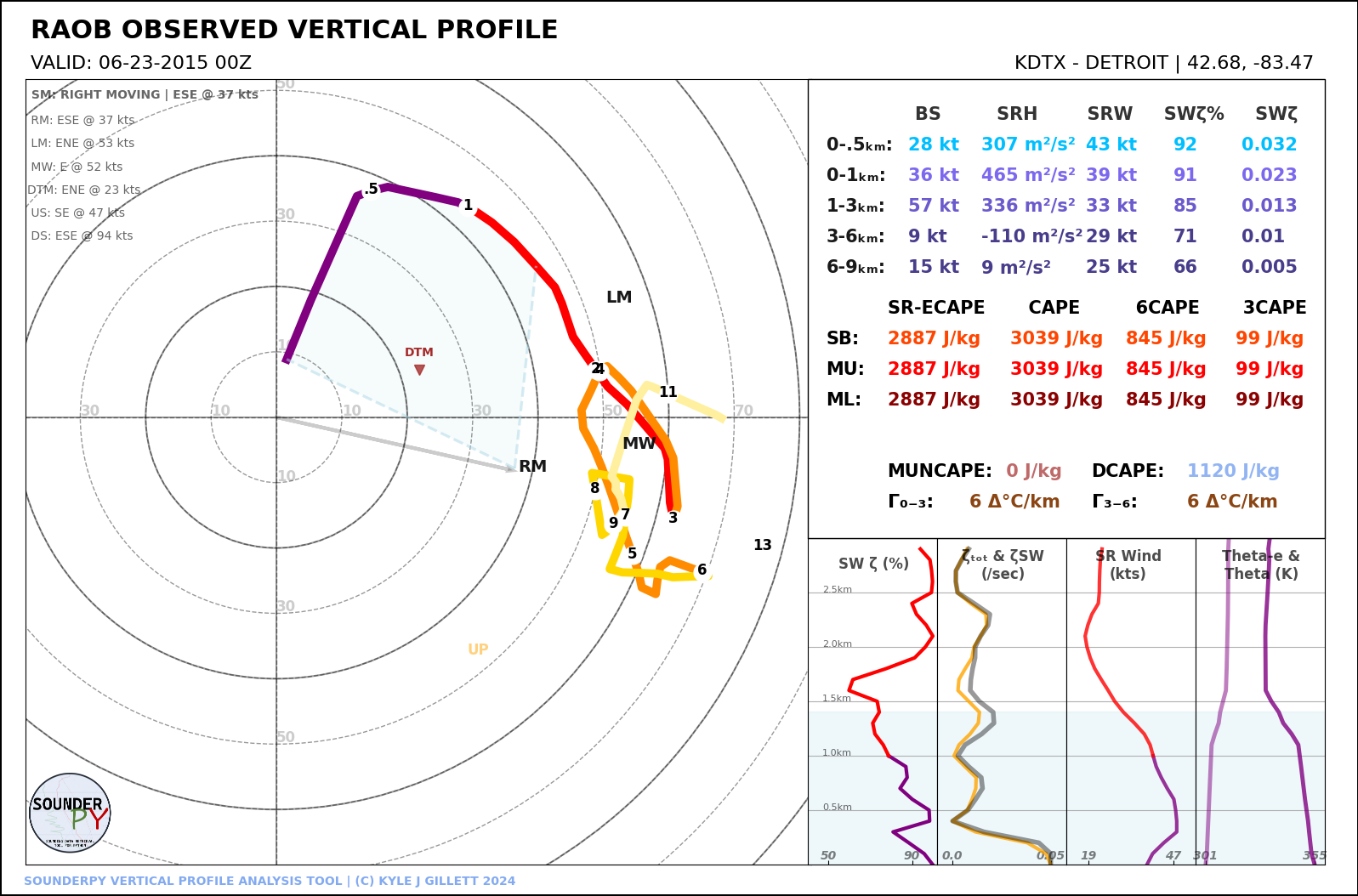
Building Hodographs
Very similarly to soundings, we can use the simple spy.build_hodograph() function:
- spy.build_hodograph(clean_data, dark_mode=False, storm_motion='right_moving', sr_hodo=False, modify_sfc=None, save=False, filename='sounderpy_sounding')
Return a full hodograph plot of SounderPy data,
plt- Parameters:
clean_data (dict, required) – the dictionary of data to be plotted (see 🌐 Tools for Getting Data)
dark_mode (bool, optional, Default is
False.) –Truewill invert the color scheme for a ‘dark-mode’ sounding.storm_motion (str or list of floats, optional, Default is 'right_moving'.) – the storm motion used for plotting and calculations. Custom storm motions are accepted as a list of floats representing direction and speed. Ex:
[270.0, 25.0]where ‘270.0’ is the direction in degrees and ‘25.0’ is the speed in kts. See the Storm Motion Logic section for more details.sr_hodo (bool, optional, default is
False) – transform the hodograph from ground relative to storm relativemodify_sfc (None or dict, optional, default is None) – a dict in the format
{'T': 25, 'Td': 21, 'ws': 20, 'wd': 270}to modify the surface values of theclean_datadict.radar (str,
"mosaic","single-site", orNone. Optional. Default ismosaic.) – whether to display mosaic reflectivity, single-site reflectivity, or no radar in the map inset.radar_time (str or datetime obj, optional, Default is
"sounding".) – radar mosaic data valid time. May be"sounding"(uses the valid time of the sounding data),``”now”`` (current time/date), or a datetime obj Note: radar mosaic data only goes back 1 month from current datemap_zoom (int, optional, Default is
2.) – a ‘zoom’ level for the map inset as an int. Note: Setting ``map_zoom=0`` will hide the maphodo_boundary (dict of lists – structured as
{'angle':[], 'color':[]}, optional) – plot a “boundary” (straight line) on the hodograph axis. Do so by providing an angle and a color. The angle represents the angle between zero-degrees (north) and the upper-half of the boundary line, to the right. Multiple boundaries can be plotted. Default isNonesave (bool, optional, Default is
False.) – whether to show the plot inline or save to a file.filename (str, optional, Default is sounderpy_sounding.) – the filename by which a file should be saved to if
save = True.
- Returns:
plt, a SounderPy hodograph figure
- Return type:
plt
Example
import sounderpy as spy

# get data | Note: any sounderpy data will work!
clean_data = spy.get_obs_data('OAX', '2014', '06', '16', '18')

# build the hodograph!
spy.build_hodograph(clean_data)
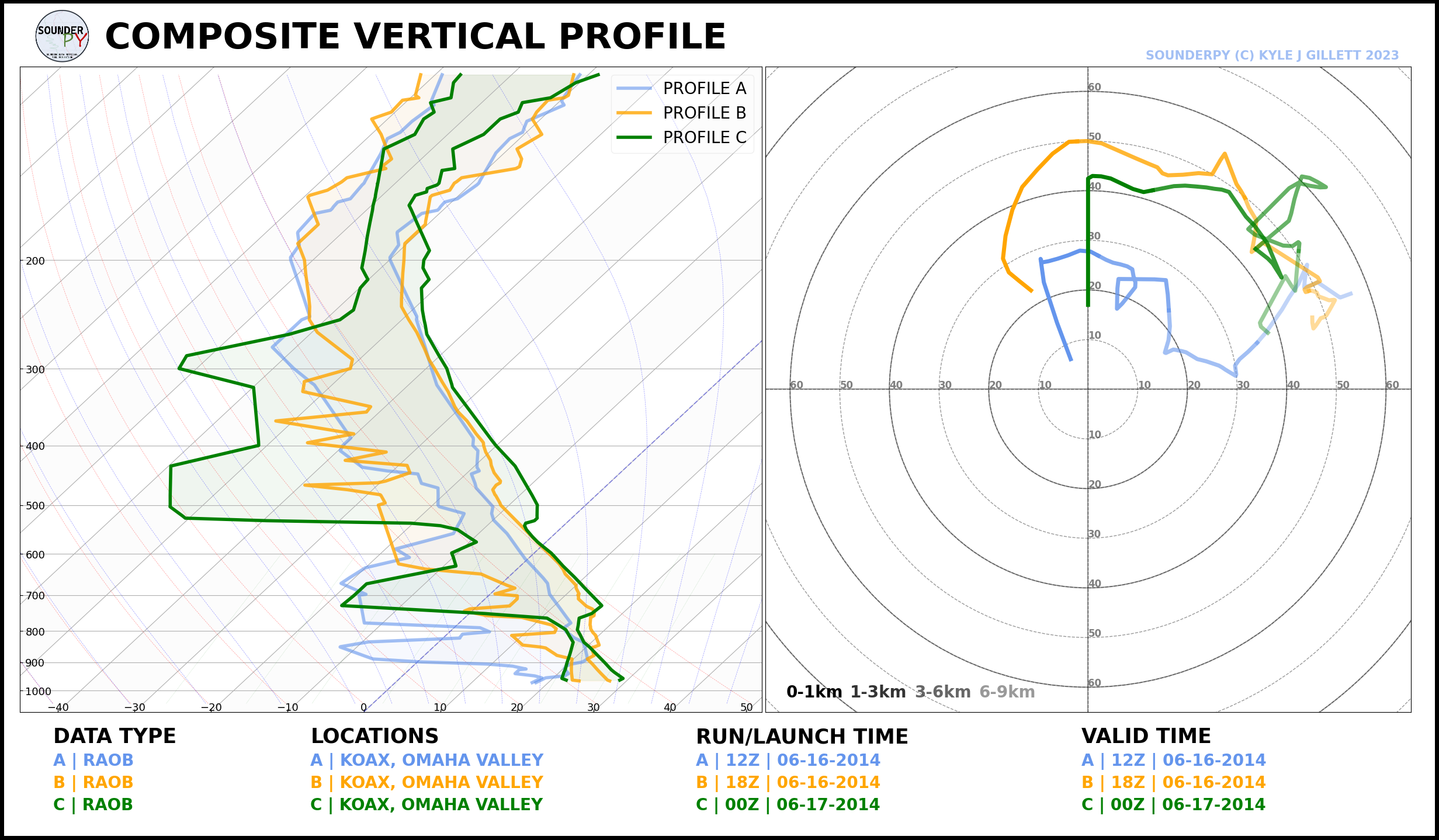
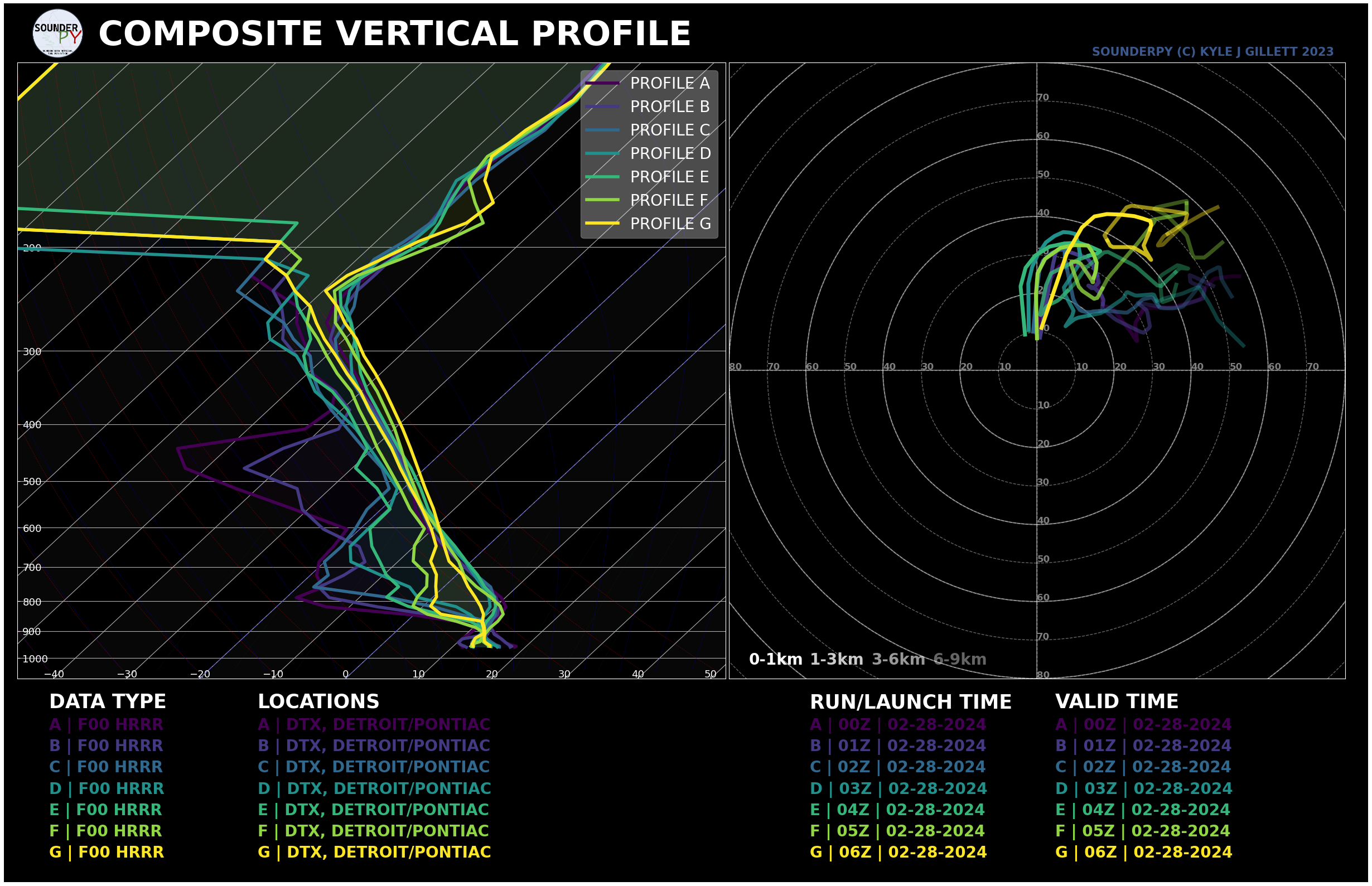
Building Composite Soundings
Sometimes we want to compare two or more profiles against each other. Perhaps at different locations or times, or we may want to compare different models or model run-times. SounderPy allows you to do this!
To do so, a list of ‘clean_data’ dicts is needed. If you want to customize the look of each profile, you can create equal length lists with alphas, linestyles, linewidths, & colors. See below:
- spy.build_composite(data_list, cmap='viridis', colors_to_use='none', shade_between=False, alphas_to_use='none', ls_to_use='none', lw_to_use='none', dark_mode=False, save=False, filename='sounderpy_sounding')
Return a composite sounding plot of multiple profiles,
plt- Parameters:
data_list (list of dicts, required) – a list of
clean_datadictionaries for each profile to be plottedshade_between (bool, optional, Default is
True.) – Lightly shade between the dewpoint & temperature trace. In many cases, this improves readability.cmap (matplotlib.colors.LinearSegmentedColormap or str representing the name of a matplotlib cmap, optional, Default is ‘viridis’.) – a linear colormap, may be any custom or matplotlib cmap. If
colors_to_usekwarg is provided,colors_to_usewill be used instead.colors_to_use (list of strings, optional, Default is 'none'.) – A list of custom matplotlib color name stings. List length must match the number of profiles listed in
data_list.alphas_to_use (list of floats, optional, Default is 'none' (sets alpha to 1)) – A list of custom alphas (0.0-1.0). List length must match the number of profiles listed in
data_list.ls_to_use (list of stings, optional, Default is 'none' (sets linestyle to '-')) – A list of custom matplotlib linestyles. List length must match the number of profiles listed in
data_list.lw_to_use (list of floats, optional, Default is 'none' (sets linewidth to 3).) – A list of custom linewidths. List length must match the number of profiles listed in
data_list.dark_mode (bool, optional, Default is
False.) –Truewill invert the color scheme for a ‘dark-mode’ sounding.save (bool, optional, Default is
False) – whether to show the plot inline or save to a file.filename (str, optional, Default is sounderpy_sounding.) – the filename by which a file should be saved to if
save = True.
- Returns:
plt, a SounderPy composite sounding figure
- Return type:
plt
Examples
import sounderpy as spy

# get data | Note: any sounderpy data will work!
# this example looks at 3 profiles from OAX on Pilger-day.
clean_data1 = spy.get_obs_data('oax', '2014', '06', '16', '12')
clean_data2 = spy.get_obs_data('oax', '2014', '06', '16', '18')
clean_data3 = spy.get_obs_data('oax', '2014', '06', '17', '00')

# add each dict of data to a list
data_list = [clean_data1, clean_data2, clean_data3]

# build the composite!
spy.build_composite(data_list)
import sounderpy as spy

# get data | Note: any sounderpy data will work!

data_list = []
for hour in ['00', '01', '02', '03', '04', '05', '06']:
    cd = spy.get_bufkit_data('hrrr', 'dtx', 0, '2024', '02', '28', hour, hush=True)
    data_list.append(cd)

# and make it dark-mode for fun!
spy.build_composite(data_list, dark_mode=True, lw_to_use=[4 for cd in data_list])
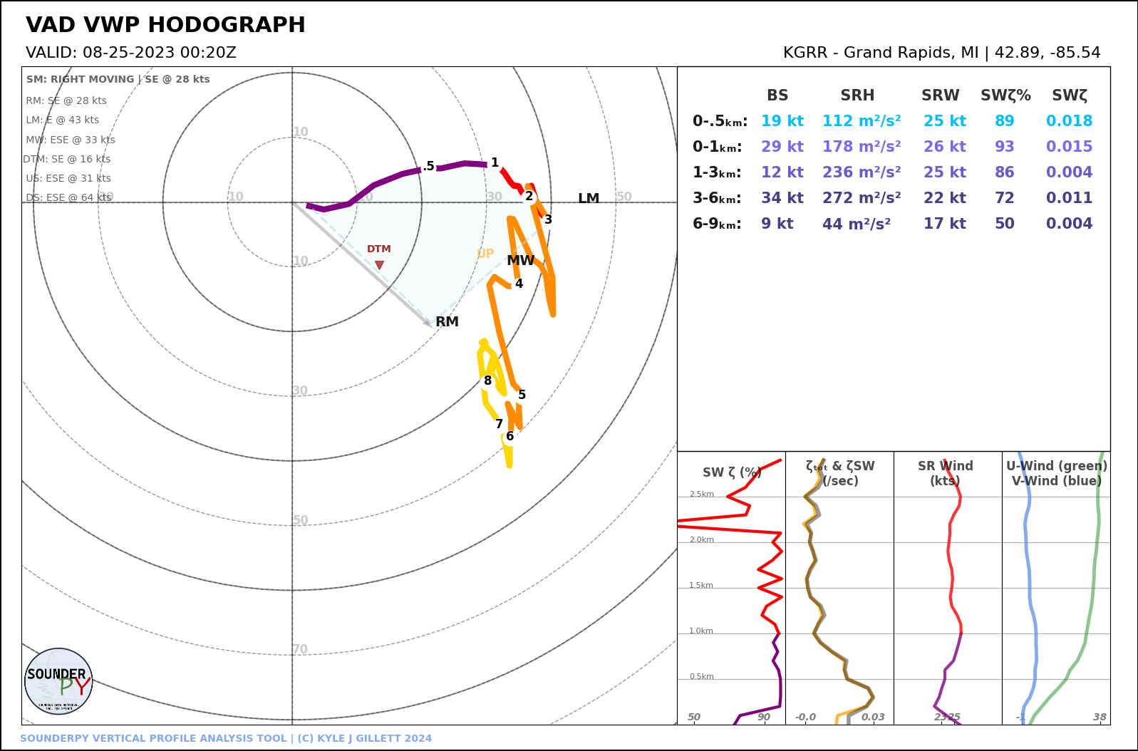
Building VAD Hodographs
Experimental function, but available for use. Errors are possible.
SounderPy now offers the ability to plot NEXRAD radar VAD data on a hodograph using the spy.build_vad_hodograph() function:
- spy.build_vad_hodograph(vad_data, dark_mode=False, storm_motion='right_moving', sr_hodo=False, save=False, filename='sounderpy_sounding')
Return a full hodograph plot of SounderPy VAD data,
plt- Parameters:
vad_data (dict, required) – the dictionary of VAD data to be plotted
dark_mode (bool, optional, Default is
False.) –Truewill invert the color scheme for a ‘dark-mode’ sounding.storm_motion (str or list of floats, optional, Default is 'right_moving'.) – the storm motion used for plotting and calculations. Custom storm motions are accepted as a list of floats representing direction and speed. Ex:
[270.0, 25.0]where ‘270.0’ is the direction in degrees and ‘25.0’ is the speed in kts. See the Storm Motion Logic section for more details.sr_hodo (bool, optional, default is
False) – transform the hodograph from ground relative to storm relativesave (bool, optional, Default is
False) – whether to show the plot inline or save to a file.filename (str, optional, Default is sounderpy_sounding.) – the filename by which a file should be saved to if
save = True.
- Returns:
plt, a SounderPy sounding built with Matplotlib, MetPy, SharpPy, & SounderPy.
- Return type:
plt
Examples
Surface Modification Logic
Users may override the zeroth (surface) value of the clean_data dict, when creating a plot or returning sounding parameters, using the modify_sfc kwarg. This argument is a python dictionary.
SounderPy takes the users requested surface modifications and preforms an “Barnes style” interpolation of the new surface values with the existing profile up several points. Please note that as of release v3.0.5, this is to be considered a “beta” version of the feature. As such, it may not always perform as expected.
The modify_sfc dict
T: Temperature, degrees Celsius
Td: Dewpoint, degrees Celsius
ws: Wind speed, knots
wd: Wind direction, meteorological degrees (north=0)Examples:
spy.build_sounding(clean_data, modify_sfc={'T':21, 'Td':19, 'ws': 30, 'wd':270})

spy.build_sounding(clean_data, modify_sfc={'T':21, 'Td':19})

spy.build_sounding(clean_data, modify_sfc={'ws': 30, 'wd':270})
Storm Motion Logic
Users can define custom storm motions or choose from a number of ‘storm motion keys’ to change the storm motion considered by kinematic and thermodynamic parameters during calculations and plotting. All parameters that consider storm motion will be affected by the storm_motion kwarg.
Storm Motion Keys
right_moving: Bunkers Right Moving supercell (default)
left_moving: Bunkers Left Moving supercell
mean_wind: 0-6km mean wind.Example:
storm_motion='left_moving'
Custom Storm Motions
Custom storm motions must be given in a list including direction in degrees and speed in knots. Note: degrees must be in the meteorological convention of ‘from’, i.e. ‘northeast’ would be 225 degrees, not 45 degrees.
Example:
# 250 degrees at 45 knots
storm_motion=[250, 45]
Parcel Logic
New to v3.0.2+, the ‘parcel-update’, is a complex scheme for computing and plotting advanced parcels using various adiabatic ascent schemes and entrainment schemes. This toolkit comes from Amelia Urquhart’s ecape-parcels Python package, which is based on work by Peters et. al. 2022.
When plotting soundings, users can choose from a number of parcel types to compute and plot, such as…
Pseudoadiabatic non-entraining ascent CAPE
Pseudoadiabatic entraining ascent CAPE
Irreversible Adiabatic non-entraining ascent CAPE
Irreversible Adiabatic entraining ascent CAPE
Each of these parcel types can be computed and plotted from a/the…
Surface-based parcel
Most-Unstable parcel
Mixed Layer parcel
How to use this feature
When plotting a full sounding using the build_sounding() function, use the kwarg special_parcels to choose which parcels you’d like to plot. This kwarg is a nested list ([[a, b], [c, d]]), where the first list contains ‘highlight’ parcels and the second list contains ‘background’ parcels. I.e., ‘highlighted’ parcels are darker and on top of ‘background’ parcels, which appear faded and behind the ‘highlight’ parcels.
Example:
special_parcels = [["sb_ia_ecape"], ["sb_ps_ecape", "sb_ps_cape"]]By default, SounderPy will plot normal MU/ML/SB-CAPE parcels and an mu_ia_ecape parcel. You can override this by setting
special_parcelsto ‘simple’, which only plots the common MU/ML/SB-CAPE parcels. This is greatly reduce the plot-time!
Parcel Keys
Note the struture of the ‘parcel key’: sb_ia_ecape. This is broken into three components: ‘parcel-type’, ‘ascent-scheme’, and ‘entrainment-scheme’. You can make any parcel you like using this specific nomenclature: parcel-type_ascent-scheme_entrainment-scheme.
PARCEL-TYPES
sb: surface-based parcel
mu: most-unstable parcel
ml: mixed-layer parcel
ASCENT-SCHEMES
ps: Pseudoadiabatic ascent
ia: - Irreversible adiabatic ascent
ENTRAINMENT-SCHEMES
cape: non-entraining convective available potential energy
ecape: entraining convective available potential energy
Examples:
'sb_ia_ecape': surface-based irreversible adiabatic entraining CAPE
'mu_ps_cape': most-unstable pseudoadiabatic CAPE
'ml_ia_cape': mixed-layer irreversible adiabatic CAPE
'sb_ps_ecape': surface-based pseudoadiabatic entraining CAPE
Radar Logic
Knowing the location of a vertical profile relative to nearby meteorological phenomenon is vital in understanding what that vertical profile means for the atmosphere at a given time. To help with this, SounderPy employs the use of mapping & radar data to provide this information to a reader.
Using the Map
The map is simply controlled by the “map_zoom” key-word-argument (kwarg) in the build_sounding() & build_hodograph() functions. Setting ``map_zoom=0`` will hide the map completely. Otherwise, map_zoom must be an int describing the size of the map. A larger int will reveal more of the map (zooming out).
Using Radar
SounderPy offers two sources of radar data to the user. First is a CONUS reflectivity mosaic, and the other is single-site NEXRAD WSR-88D reflectivity. The CONUS mosaic is default because its fastest and easiest to plot, but data availablity is only up to 30 days before the current date. Single-site radar goes back much further but data availability varies by site and date.
To plot radar on a sounding or hodograph, there are two kwargs to understand:
radar
"mosaic": plots the CONUS reflectivity mosaic
"single": plots single-site WSR-88D reflectivity closest to the latitude/longitude coordinates of the sounding.
radar_time
"now": plots the most recent radar scan
"sounding": plots the radar scan closest the time of the sounding
datetime(1999, 5, 4, 0, 27): or you may define your own time by providing a datetime obj. This will plot the nearest radar scan to the date/time provided.
About These Plots
This plot style has been developed in a way that acts to provide as much information to the user as possible with attributes designed specifically for the analysis of severe convective environments, and supercells/tornadoes in particular. You will also find that this particular plot style does not host many of the common and popular severe weather composite indices – that was intentional. Most, if not all, of the data provided on this plot, are considered, for the lack of a better word, ‘true’ observations of the atmosphere though most are still subject to heavy assumptions.
The data on these plots are considered, by most, to be useful in determining critical characteristics of the atmosphere related to supercellular storm mode and tornadogenesis.