Creating Sounding Plots

This tutorial creates SounderPy Sounding plots!

Here we will explore:

• Full Soundings

• Plots in Dark Mode

• Color blind friendly settings

• Saving soundings to a file

# First lets import SounderPy. Its fun to import as 'spy'!
import sounderpy as spy

## ---------------------------------- SOUNDERPY ----------------------------------- ##
##          Vertical Profile Data Retrieval and Analysis Tool For Python            ##
##                     v3.0.5 | Sept 2024 | (C) Kyle J Gillett                      ##
##                 Docs: https://kylejgillett.github.io/sounderpy/                  ##
## --------------------- THANK YOU FOR USING THIS PACKAGE! ------------------------ ##

Load some data to plot

Here we can load some data with SounderPy.

Let’s investigate OUN (Norman, OK) observations for El-Reno 2013. We can use the get_obs_data() function to do this

clean_data = spy.get_obs_data('oun', '2013', '05', '31', '18')

> OBSERVED DATA ACCESS FUNCTION
  -----------------------------------
    > PROFILE FOUND: OUN on 05/31/2013 at 18z | From UW
    > COMPLETE --------
    > RUNTIME: 00:00:03
    > SUMMARY: 18Z Launch for KOUN, NORMAN at 05-31-2013-18Z

    > THERMODYNAMICS ---------------------------------------------
    --- SBCAPE: 5232.3 | MUCAPE: 5232.3 | MLCAPE: 4032.7 | MUECAPE: 3612.2
    --- MU 0-3: 131.9 | MU 0-6: 1135.3 | SB 0-3: 131.9 | SB 0-6: 1135.3

    > KINEMATICS -------------------------------------------------
    --- 0-500 SRW: 24.8 knot | 0-500 SWV: 0.011 | 0-500 SHEAR: 9.0 | 0-500 SRH: 60.2
    --- 1-3km SRW: 17.0 knot | 1-3km SWV: 0.005 | 1-3km SHEAR: 16.2 | | 1-3km SRH: 69.7
    ==============================================================

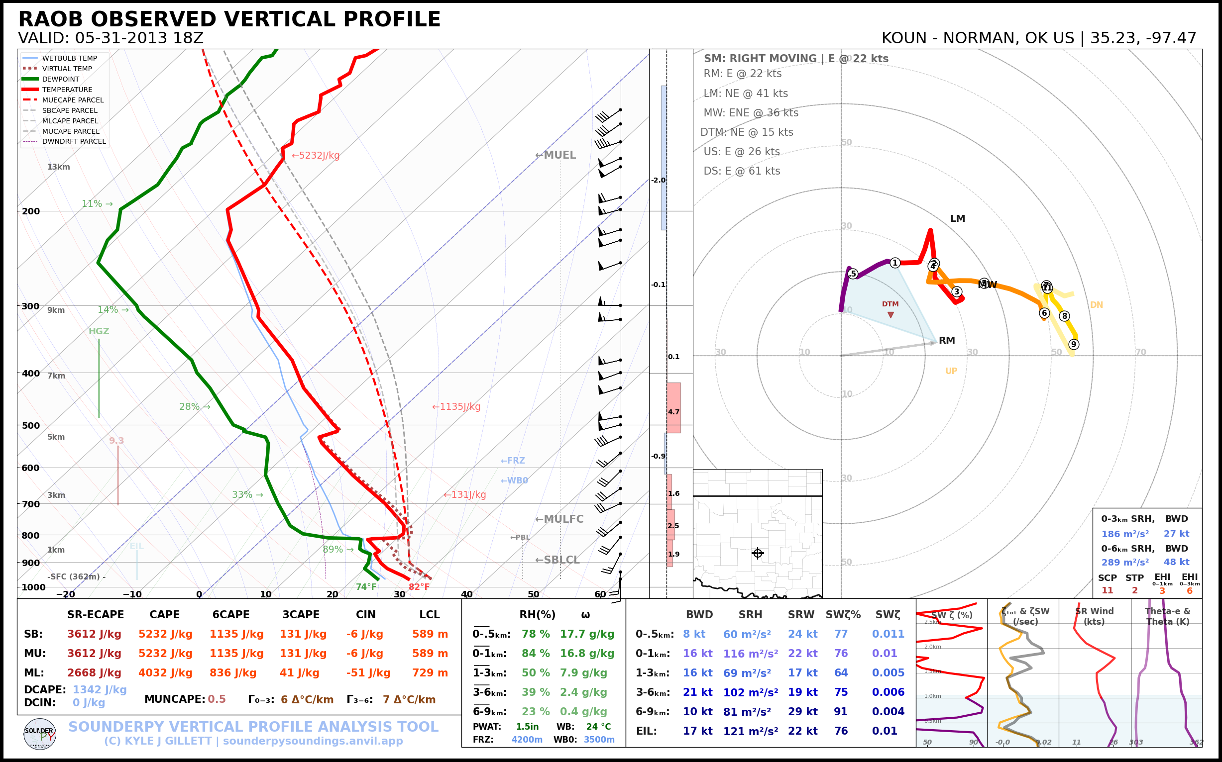
Build a full sounding plot

Here we use the most basic version of the build_sounding() function to build a ‘full sounding’. Making a SounderPy sounding figure is as simple as:

# lets make a full sounding!
spy.build_sounding(clean_data)

> SOUNDING PLOTTER FUNCTION
  ---------------------------------
- no radar data available -
    > COMPLETE --------
    > RUNTIME: 00:00:23

Playing with sounding settings

Now we can adjust a few settings to customize the plot a little bit.

To do so, let’s first study the build_sounding() function…

build_sounding(clean_data, color_blind=False, dark_mode=False, storm_motion='right_moving', special_parcels=None, modify_sfc=None, show_radar=True, radar_time='sounding', map_zoom=2, save=False, filename='sounderpy_sounding')

where:

• clean_data (dict, required) – the dictionary of data to be plotted

• color_blind (bool, optional) – whether or not to change the dewpoint trace line from green to blue for improved readability for color deficient users/readers. Default is False

• dark_mode (bool, optional) – True will invert the color scheme for a ‘dark-mode’ sounding. Default is False.

• storm_motion (str or list of floats, optional) – the storm motion used for plotting and calculations. Default is ‘right_moving’. Custom storm motions are accepted as a list of floats representing direction and speed. Ex: [270.0, 25.0] where ‘270.0’ is the direction in degrees and ‘25.0’ is the speed in kts.See the documentation for more details.

• special_parcels (nested list of two lists, optional) – a nested list of special parcels from the ecape_parcels library. The nested list should be a list of two lists ([[a, b], [c, d]]) where the first list should include ‘highlight parcels’ and second list should include ‘background parcels’. Another option is ‘simple’, which removes all advanced parcels making the plot quicker. See the documentation for more details.

• save (bool, optional) – whether to show the plot inline or save to a file. Default is False which displays the file inline.

• filename (str, optional) – the filename by which a file should be saved to if save = True. Default is ‘sounderpy_sounding’.

• show_radar (bool, optional, Default is True) - whether or not to display mosaic radar data on the map inset.

• radar_time (str, optional, Default is sounding.) - radar mosaic data valid time. May be sounding (uses the valid time of the sounding data), or now (current time/date). Note: radar mosaic data only goes back 1 month from current date

• map_zoom (int, optional, Default is 2.) - a ‘zoom’ level for the map inset as an int. Note: Setting ``map_zoom=0`` will hide the map

• modify_sfc: (None or dict, optional, default is None) - a dict in the format {'T': 25, 'Td': 21, 'ws': 20, 'wd': 270} to modify the surface values of the clean_data dict. See the documentation for more details.

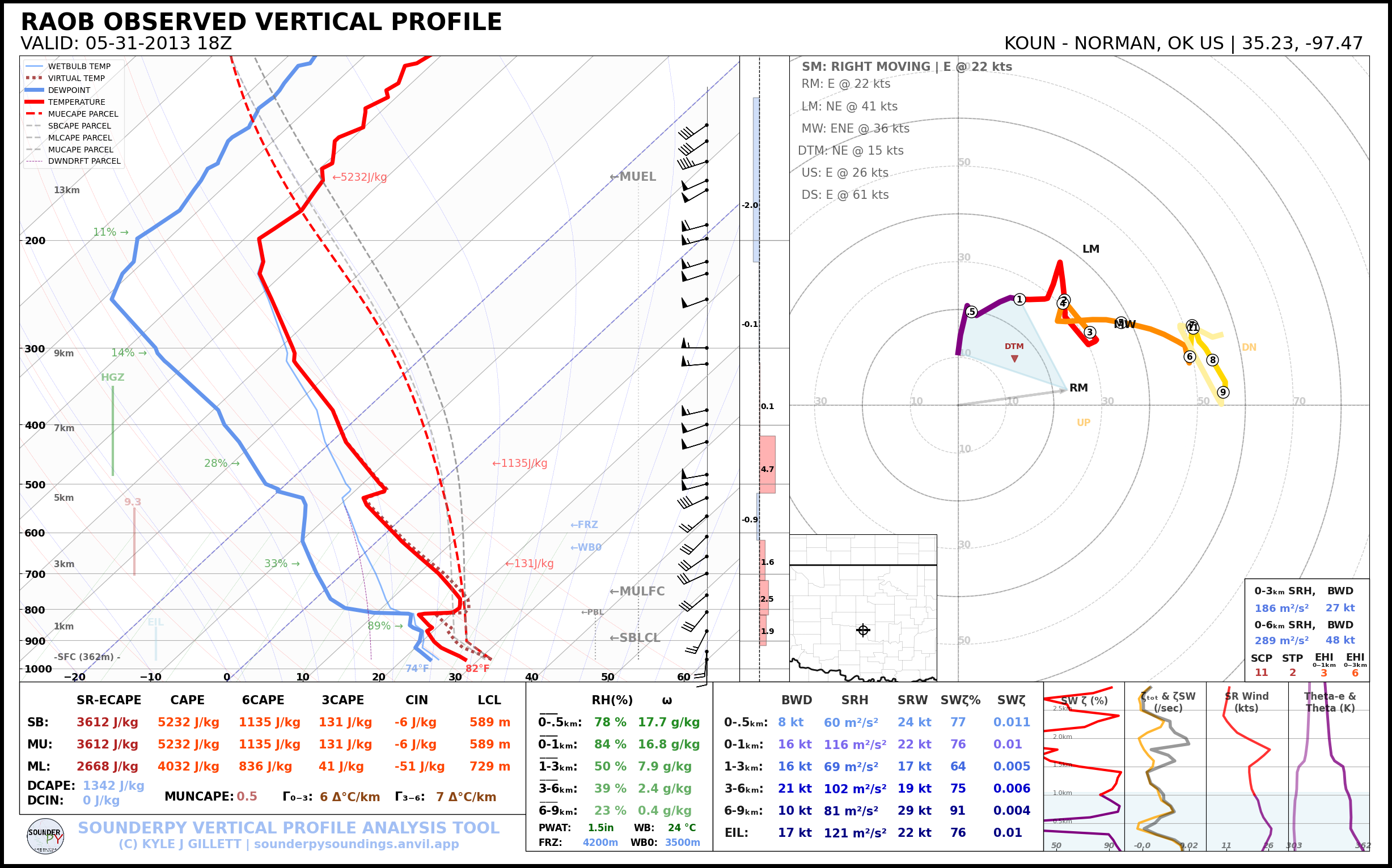
Lets try the color_blind setting:

# color_blind turned on!
spy.build_sounding(clean_data, color_blind=True)

> SOUNDING PLOTTER FUNCTION
  ---------------------------------
- no radar data available -
    > COMPLETE --------
    > RUNTIME: 00:00:15

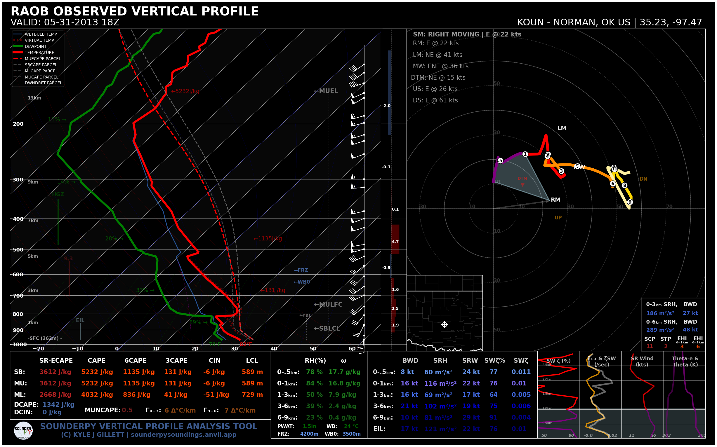
And now, for probably the coolest part: dark mode!

# dark_mode turned on!
spy.build_sounding(clean_data, dark_mode=True)

> SOUNDING PLOTTER FUNCTION
  ---------------------------------
- no radar data available -
    > COMPLETE --------
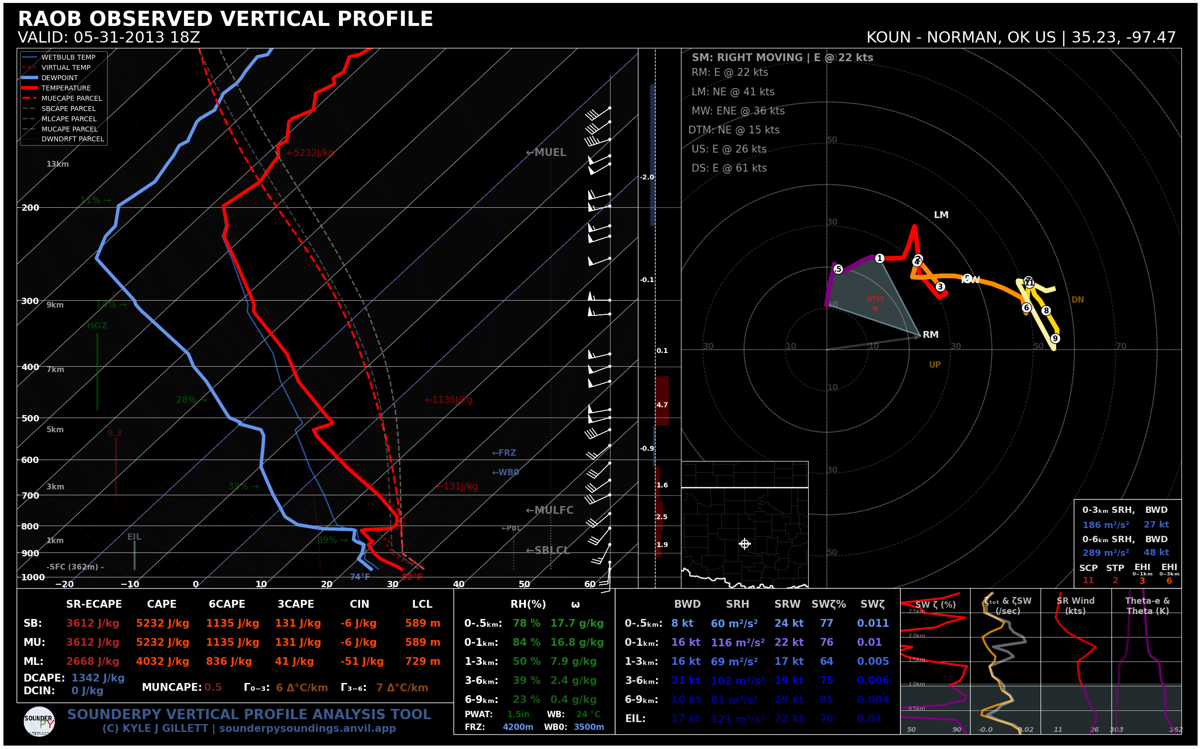
    > RUNTIME: 00:00:16

# dark_mode and color_blind turned on!
spy.build_sounding(clean_data, dark_mode=True, color_blind=True)

> SOUNDING PLOTTER FUNCTION
  ---------------------------------
- no radar data available -
    > COMPLETE --------
    > RUNTIME: 00:00:14

Saving plots as a file

By default, SounderPy is set to show plots inline. If you want/need to save them to a file, SounderPy offers that option!

Just set the save kwarg to True, and give it a file name using the filename kwarg!

IMPORTANT NOTE!!!

• If your plots come out with a funky layout when displaying them inline, it may be due to your screen resolution.

• In the event that this is the case, simply use the save=True option to save plots to a file!

#spy.build_sounding(clean_data, save=True, filename='sounderpy_2013051318z_OUN')